
1. Introduction
In spoken language interactions, speech sounds must be perceptually categorized consistently across talkers for these to understand each other. One key objective in speech communication research is to explain how people can perceive speech sounds in a way that is similar enough to ensure mutual understanding. To achieve this remarkable feat, talkers must share a set of conventions on how to map speech sounds onto linguistically relevant categories.1 These conventions result from countless inter-individual interactions over entire generations of talkers, which resonate within each individual whenever she recognizes a vowel or consonant in the speech stream. The goal of this study was to contribute to the characterization of the cognitive mechanisms that preside over the formation of this shared perceptual space.
Computational models of the emergence of language (e.g., De Boer, 2000; Moulin-Frier et al., 2015) have shown that speech sound systems can arise at a collective scale as the byproduct of pairwise communication between agents. According to these models, local, unidirectional or bidirectional communicative exchanges engender the gradual formation of a globally shared speech code. In the COSMO model (Moulin-Frier et al., 2015) for example, a common repertoire of linguistic units for referring to objects progressively forms itself in a group of communicating agents through sequences of sensorimotor operations performed by pairs of agents. Likewise, in De Boer’s (2000) model, vowel systems emerge by virtue of a self-organization process from pairwise interactions between agents, each of which has to imitate the sounds produced by the other. In the experimental domain, researchers have used innovative designs to identify the conditions that may account for the emergence of language (Scott-Phillips & Kirby, 2010; Verhoef et al., 2014) and these researchers too regard pairwise communicative exchanges as the building blocks upon which linguistic systems can deploy themselves. This study was carried out in the framework of a project that seeks to determine how shared conventions may arise in the perception of speech as a result of inter-individual communicative exchanges. We more specifically aimed to answer the following question: When communicating with one another, to what extent do people converge towards each other in the way they categorize speech sounds?
Much attention has been paid over the last two decades or so to inter-individual adaptation mechanisms in the production and perception of speech. One key mechanism is phonetic convergence, i.e., the tendency for a talker to partly imitate another person’s way of producing speech sounds when exposed to that person’s speech (Babel, 2011). Ever since Goldinger’s (1998) and Pardo’s (2006) seminal studies, phonetic convergence effects between speakers have been explored in both interactive (e.g., Abel & Babel, 2016; Kim et al., 2011; Pardo, 2006) and non-interactive, laboratory (e.g., Delvaux & Soquet, 2007; Goldinger, 1998; Nielsen, 2011) settings, by means of direct, acoustic measures (e.g., Harrington et al., 2019; Mukherjee et al., 2019; Zellou et al., 2016), indirect, perceptual evaluations performed by listeners (Dias & Rosenblum, 2016; Miller et al., 2013; Pardo, 2006), or both (e.g., Clopper & Dossey, 2020; Pardo et al., 2013a, 2013b; see Pardo et al., 2017, for a review). Convergence effects in a talker as a consequence of her being exposed to other people’s speech may extend well beyond that exposure across the talker’s lifetime (Harrington et al., 2000), and it has also been assumed to play a central role at yet a larger time scale in the emergence and evolution of phonological systems (see Nguyen & Delvaux, 2015, for a review). A central issue for the present study is whether convergence in speech production entails convergence in perception. In Pickering and Garrod’s integrated theory of language production and comprehension (Pickering & Garrod, 2013, 2021), imitating the interlocutor’s way of speaking contributes to making it easier to understand what that person is saying and to predict what she will say next. It may be assumed that convergence between talkers in production causes each talker to become more attuned to the phonetic characteristics of words produced by the other talker, via a perception-action resonance phenomenon. However, whether this may result in both talkers categorizing speech sounds in a more similar manner appears to remain an open question.
To study convergence in perception as a potential correlate of convergence in production, experiments must by definition combine convergence-in-production with convergence-in-perception tasks. To our knowledge, there have been very few studies in that category. Adank et al. (2010) exposed Dutch-speaking participants to a novel, artificially-created accent under different conditions during a training phase, and assessed comprehension of the accent before and after training (by measuring the signal-to-noise ratio at which listeners could repeat 50% of the key words in sentences heard with background noise). The results showed that accented speech comprehension was improved after training for participants whose task was to imitate the speaker’s accent in the training phase (but not for those who had to listen to the accented sentences, or to listen and transcribe them, or to listen and repeat them in the participant’s own accent, during training). In Nguyen et al.’s (2012) experiment, however, phonetic imitation did not have a significant impact on how listeners later recognized words in a non-native regional accent. The authors suggested that phonetic convergence may contribute to predicting upcoming words in sentences in adverse listening conditions, in accord with Adank et al.’s (2010) findings, but may play a more limited role in the recognition of single words. Importantly, both Adank et al.’s (2010) and Nguyen et al.’s (2012) studies examined whether phonetic convergence towards a model speaker can facilitate understanding that speaker, but did not ask whether convergence in production implies, or is conducive to, convergence in perception.
In recent work, Lancia & Nguyen (2019) and Huttner & Nguyen (2023) explored potential convergence effects in perception from a different angle. In both studies, the authors’ goal was to find a way to provoke these effects regardless of whether they may or may not be connected with convergence in overt production. To do this, the authors used a joint-perception paradigm. Participants were asked to perform a phoneme identification task in a joint fashion and were explicitly instructed to respond in the same way as their partner(s). On each trial, each participant first responded individually to the stimulus, then was shown the response(s) of the other participant(s). The results showed that participants tended to increasingly agree with each other on how to categorize the stimuli as the experiment unfolded.
Joint perception appears to be a still developing field, but a very promising one. It has been mostly explored in the visual domain (Bahrami et al., 2010; Koriat, 2012; Richardson et al., 2012; Seow & Fleming, 2019; Sorkin et al., 2001; Wahn et al., 2018). In these studies, one of the main objectives has been to determine whether “two heads are better than one”, i.e., to what extent two people that communicate with each other do better than individuals in perceptual decision-making tasks (Bahrami et al., 2010; Koriat, 2012; Sorkin et al., 2001) and, for more than two people, whether there is a group benefit in the accomplishment of these tasks (Wahn et al., 2018). Another central objective is to characterize the effect of social context on perceptual decision-making (Richardson et al., 2012; Seow & Fleming, 2019), in a perspective that can be traced back to Asch’s (1951) landmark work. These studies all used tasks in which responses, whether produced by one or more people, can be classified as correct or incorrect. In Bahrami et al. (2010) for example, participants judged which of two briefly presented visual stimuli contained an oddball target. Lancia & Nguyen (2019) and Huttner & Nguyen (2023) applied the joint-perception paradigm to speech in a way that is novel in two respects: First, they extended this paradigm to perception of auditory speech. Second, and in both studies, pairs of participants were presented with speech sounds that ranged on an acoustic continuum between two endpoints associated with two different phonemic categories (/s/ and /ʃ/), as in a standard phoneme identification task. In such a task, and as is well known, stimuli between the two endpoints are perceived as ambiguous to various degrees, and there is no a priori correct response. These two studies therefore did not aim to determine whether performance increased when listeners did the task in pairs rather than individually. Rather, they asked to what extent two listeners can come to use the same criteria in mapping speech sounds onto phoneme categories.
Our research project stands across the modeling and experimental domains. We aim to develop a Bayesian model of convergence between listeners in speech perception, which we put to the test using novel experimental designs. The present work formed a first step towards this goal.
In the next three sections, we first lay out an initial version of the model (Section 2) and the predictions that can be made from it (Section 3). We then present our experiment (Section 4), which, building on Lancia & Nguyen (2019), entailed participants performing a joint phoneme identification task with a partner. Unlike in this previous study, however, and unbeknownst to the participants, their partner was an artificial agent whose responses we manipulated in order to examine their effects on the participants’ own responses. Our results are presented in Section 5. This is followed by the presentation of a set of simulations that we conducted with a view to accounting for these results (Section 6), and a general discussion (Section 7).
2 Towards modeling convergence between listeners in speech perception
2.1 Theoretical background
As already indicated, we have undertaken to design our model in a Bayesian framework. Bayesian models, in the study of cognition and of the human brain in general, have had widespread application and success in the last decades. They are found at most description levels, from probabilistic computational neuroscience (e.g., Friston, 2010; Pouget et al., 2013), to probabilistic models implementing psychologically based or neuro-plausible theories of sensory processing (e.g., Chikkerur et al., 2010; Ginestet et al., 2022; Laurent et al., 2017; Yu et al., 2009), to computational-level accounts of cognitive functions (e.g., Brainard & Freeman, 1997; Kersten et al., 2004; Weiss et al., 2002). They even connect seamlessly, and sometimes are close mathematical cousins to statistical methods and tools (e.g., Clayton, 2021; Dayan & Abbott, 2001; Ma, 2012). They have also percolated through almost all subdomains of cognitive science, concerning most if not all sensory modalities and their combinations (e.g., Alais & Burr, 2004; Ernst & Banks, 2002; Geisler, 2008; Mamassian et al., 2003; Weiss et al., 2002; Wozny et al., 2008; Yuille & Kersten, 2006; Zupan et al., 2002), abstract reasoning and learning (e.g., Chater et al., 2010; Tenenbaum et al., 2011), metacognition (Fleming & Daw, 2017), motor control (e.g., Patri et al., 2018; Wolpert, 2007; Wolpert & Ghahramani, 2000). Whatever their epistemological or ontological flavors, the common denominator of Bayesian models of cognition is their use of probabilities to model uncertain knowledge of the cognitive agent, and the use of Bayesian inference to model reasoning in the presence of incomplete and uncertain information (Bessière et al., 2013; Jaynes, 2003). Such characteristics can be considered as key to model human or animal cognition, which have to reason with incomplete and uncertain knowledge. In the field of speech and language, work by Norris & McQueen (2008) and Norris et al. (2016) (speech recognition), Sohoglu & Davis (2020) (brain underpinnings of speech perception), Xu & Tenenbaum (2007) (word learning), Carr et al. (2020) (language evolution), and Moulin-Frier et al. (2015) (emergence of phonological systems), among others, have shown the fertility of Bayesian approaches and the broad perspectives they offer.
In their application to speech, Bayesian approaches allow us to model phoneme identification as a probabilistic process that mathematically takes into account sensory and categorical uncertainty. They also make it possible to evaluate to what extent the listener’s prior beliefs come into play in her decision-making, along with the perceptual evidence that is available to her. In addition, and because Bayesian models, in essence, boil down to updating prior beliefs in the face of the available evidence, they are well fitted to modeling adaptation and learning processes. These are all characteristics that, in our view, are relevant to speech perception.
Our current model draws on previous work by Feldman et al. (2009), Kronrod et al. (2016) and Kleinschmidt & Jaeger (2015) (see also Clayards et al., 2008; Kleinschmidt, 2020). These models aim to account for how individual listeners identify speech sounds equally spaced along an acoustic dimension between two endpoints respectively and unambiguously associated with two phonemic categories in a two-alternative forced choice (2AFC) task. Taking these models as a starting point, we propose a simple extension to joint perception in dyads of listeners. In this first step, our goal is to model the listeners’ asymptotic behavior. More specifically, we seek to determine the extent to which listeners may perceptually converge towards their partners, from the listeners’ entire set of responses. We do not endeavor yet to model trial-by-trial changes in the listeners’ response pattern.
2.2 The single-listener model
Like most Bayesian models of perception (Gifford et al., 2014; Ma et al., 2023; Vincent, 2015), ours has a generative (forward) component and an inferential (inverse) component. The generative component contains a characterization of how sounds distribute themselves in the acoustic domain for each category. This is specified by two conditional probability distributions, p(S|c1) and p(S|c2), where S refers to a representation of the acoustic space and c1 and c2 to the two categories, respectively. It is usually assumed that p(S|c1) and p(S|c2) are both normal distributions and, when S is assumed to be monodimensional, as is generally the case in 2AFC tasks, are each characterized by a mean and a variance:
For each distribution, variance is a sum of two terms, , a measure of dispersion of the intended target sound around the mean for the category, and , which represents articulatory, acoustic and perceptual noise around the intended target sound independent of the category (Feldman et al., 2009; Kronrod et al., 2016).
As in both Feldman et al. (2009) and Kleinschmidt & Jaeger (2015), the variances associated with the two categories are considered as equal:
We further assume that the two distributions are in symmetric positions with respect to the midpoint of the continuum,2 i.e., at the same distance δµ from that midpoint, on either side of it. Both distributions are schematized in the middle panel of Figure 1.

Figure 1: Three main components of the single-listener model. Left panel: Bernoulli distribution associated with the prior probabilities p(c1) and p(c2) for the two phonemic categories. The two prior probabilities are here assumed to be equal, i.e., p(c1) = p(c2) = 0.5. Middle panel: Distributions of sounds in a one-dimensional acoustic space S for the two categories. Voice Onset Time (VOT), as one of the main acoustic cues to the /b/-/p/ phonemic contrast, is used here as the example for S. The /b/ category corresponds to shorter VOT values (on the left of the continuum) and the /p/ category to longer VOT values. Right panel: Posterior probability value for c1, given the sound. Figure partly made using the R script associated with Kurumada & Roettger (2022) and available at https://osf.io/b75q9/.
The generative component also includes the prior probabilities p(c1) and p(c2) for the two categories. This represents the listener’s prior beliefs, i.e., to what extent she expects the input sound to correspond to one category rather than the other, before hearing that sound. The prior probability can be related to the phoneme’s frequency of occurrence, among many other factors. Since there are two categories only, the prior follows a Bernoulli distribution Ber(p), i.e., p(c1) = p and p(c2) = 1 – p with 0 ≤ p ≤ 1 (see Figure 1, left panel).
The model’s inferential component allows the probability value for each phoneme category given the input sound to be computed. This is done thanks to Bayes’ theorem:
which simplifies to (Feldman et al., 2009; Kleinschmidt & Jaeger, 2015):
where, under both the same-variance and same-distance-from-mean assumptions (see Appendix 1 for further detail):
The posterior p(c1|S) thus takes the form of a logistic function governed by two parameters, g and b, as illustrated in the right panel of Figure 1. The location of the categorical boundary along the continuum is given by b/g, and the slope3 of the logistic curve at this location is given by g/4. As we posit that μ1 is lower than μ2 and therefore that μ1 – μ2 is negative, so is g, and p(c1|S) decreases as S gets closer to the endpoint associated with c2.
The logistic curve gets steeper when the normal distributions for the two phoneme categories are further apart from each other (larger difference between μ1 and μ2) and/or when these distributions are both narrower (lower category variance and/or lower noise variance ). The parameter b assimilates to a log odds ratio, and is a measure of the relative prior probabilities of the two phoneme categories. When p(c2) increases relative to p(c1), this causes the categorical boundary to be shifted towards the c1 endpoint, i.e., corresponds to a greater bias for associating the input sound with c2. In the following, we will refer to g as the Slope4 parameter and to b as the Bias parameter.
2.3 Extension to modeling perceptual convergence between listeners
We now turn to how this single-listener model can be extended to account for potential perceptual convergence effects across listeners. This is done in the context of a 2AFC phoneme identification task that is jointly performed by two listeners. On hearing each stimulus, listeners must try to predict their partner’s response and respond in the same way. Once both have responded, each listener’s response is communicated to the other listener. In such a task, we simply assume that each listener expects the other listener to behave like a Bayesian agent, and will undertake to infer the parameter distributions of her partner’s internal model, so as to get her own model to fit these distributions as well as possible. Inference is performed by each listener from the partner’s set of responses, and entails computing estimated distributions for both the Slope and Bias parameters.
For the listener, estimating the distribution of the Bias parameter amounts to asking herself whether her partner has a bias towards choosing one response over the other and, if so, which response and to what extent. To our knowledge, this issue has not been explored in previous work. There is, however, an extensive literature on post-perceptual biases in phoneme categorization tasks, on which we may rely to further characterize the potential impact of bias in our proposed experimental setting. In particular, both Connine & Clifton (1987) and Pitt (1995) examined to what extent listeners were influenced by monetary payoff, by attributing them a reward or penalty depending on which phoneme category they chose in response to each stimulus. Connine & Clifton (1987) and Pitt (1995) both found that the location of the categorical boundary shifted in accordance with monetary payoff. Because monetary payoff is an unequivocally post-perceptual bias and, in a joint phoneme categorization task, the partner’s bias can also be viewed as a post-perceptual one, links can be drawn between our experimental set-up and that of Connine & Clifton (1987) and Pitt (1995), which we further develop below.
As indicated above, the Slope parameter depends on both the means of the normal distributions for the two phoneme categories and their variance, itself an addition of the category variance and noise variance. In the process of inferring phoneme categories from sounds, noise variance relates to trial-to-trial differences in the location of the stimulus in the acoustic space as perceived by the listener. It has been pointed out (e.g., Kapnoula et al., 2017; McMurray, 2022) that the 2AFC task does not allow noise variance to be disentangled from category variance, because listeners are requested to respond in a binary fashion. In our model, as in those proposed by Feldman et al. (2009), Kleinschmidt & Jaeger (2015) and Kronrod et al. (2016), category and noise variance are not estimated independently of each other. In a joint 2AFC task, therefore, we may seek to determine to what extent each listener is sensitive to noise+category variance as a whole, as reflected in the other listener’s response pattern.
McMurray (2022) underlines that categorical perception has long been seen as being characterized by a steep identification curve and that shallower curves were seen, by contrast, as indicative of decreased precision in listeners, due to an increased amount of sensory noise. Contrary to this traditional view, however, Kong & Edwards (2016), Kapnoula et al. (2017), and Ou et al. (2021), among others, have argued that phoneme identification is intrinsically gradient and that gradiency contributes to making the speech perception system more efficient. It allows listeners to commit themselves to one phoneme category to a lesser degree in the face of more ambiguous stimuli, and make listeners more receptive to secondary cues to a phonemic contrast.
In that respect, Clayards et al.’s (2008) study is particularly relevant to our own piece of work. These authors asked to what extent listeners are sensitive to the variance of the probability distributions for voice onset time (VOT) as an acoustic cue to the voicing contrast, in word-initial bilabial voiced (e.g., beach) and voiceless (e.g., peach) stops. They exposed listeners to stimuli ranging on a VOT continuum between a voiced and a voiceless bilabial stop, and whose relative frequency of occurrence mirrored a mixture of two Gaussian distributions associated with the voiced and voiceless categories, respectively. Clayards et al. (2008) manipulated the variance of these distributions, which was either wide or narrow. In a Bayesian framework, as adopted by these authors, this amounted to manipulating the variance of the distributions p(S|c1) and p(S|c2) as defined above, where c1 and c2 refer to the voiced and voiceless stops, respectively. In accordance with the application of Bayes’ theorem in the model, the posterior categorization curve p(c1|S) was expected to be shallower in the wide-variance compared with the narrow-variance condition. Two groups of listeners performed a word-to-picture matching task in the wide-variance condition for one group and the narrow-variance condition for the other group, and their identification curves were consistent with this prediction.
In Clayards et al. ‘s (2008) study, the identification task was accomplished individually by each listener, and the variable of interest was the probability distribution of the stimulus in the acoustic space for each phoneme category. Our own focus is different and concerns the listener’s potential sensitivity to the probability distributions that may underlie another listener’s response pattern. However, Clayards et al.’s findings are of particular interest to us as they show that the listeners’ degree of gradiency, or steepness as referred to here, is flexible and may change in an adaptive way and over a short time frame. Detail about Clayards et al.’s model parameters and obtained effect size is given in Appendix 2. In the following section, we present our experimental design and predictions.
3 Experimental design and predictions
Our main goal was to determine to what extent listeners are sensitive to their partner’s bias and degree of gradiency in a joint phoneme identification task. More specifically, we sought to establish whether listeners would converge towards their partner in either or both of these two dimensions. To shed light on this issue, and unbeknownst to them, each participant performed the task not with another human participant, but with a virtual agent (a bot, hereafter). This allowed us to manipulate the bot’s response pattern in a systematic way and to examine to what extent these manipulations were mirrored in the participants’ own response patterns.
Each of the two parameters took either of two values: Steep or Shallow for the Slope parameter, biased towards one or the other of two categories for the Bias parameter. This yielded four experimental conditions, which are illustrated in Figure 2. There were four groups of participants, one for each condition. As also indicated in this figure, our experiment focused on the perception of the voicing contrast in stimuli ranging on a VOT continuum between a voiced bilabial stop and a voiceless one in syllable-initial position.
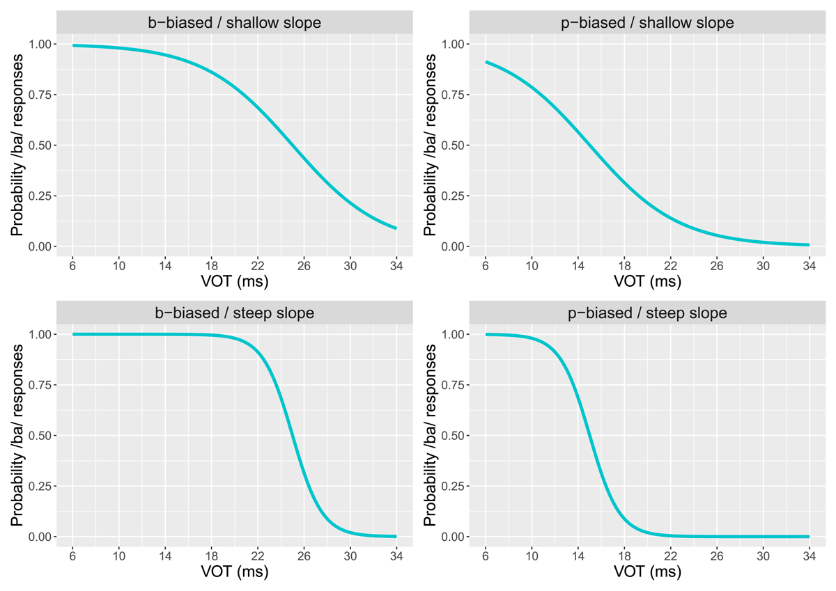
Figure 2: Bot’s schematized response patterns in the four experimental conditions. Each plot shows the bot response probability for category c1, p(c1|S) (vertical axis) as a function of VOT on the /ba/-/pa/ continuum (horizontal axis). Categories c1 (/b/) and c2 (/p/) are associated with short and longer VOT values, respectively.
We put three main predictions to the test. Our first prediction was that participants would show a stronger bias towards the voiced category in the Voiced-Biased conditions compared with the Voiceless-Biased conditions. Our second prediction was that the slope of the participants’ identification curves would be shallower in the Shallow conditions compared with the Steep conditions.
Our third prediction related to the link between Bias, on the one hand, and gradiency, on the other hand, in the setting of the location of the categorical boundary. As specified above (in 2.2), the location of the categorical boundary is given by the Bias-to-Slope ratio b/g. This means that, for the boundary to be shifted over a given interval across the continuum, Bias b must be modified to a lesser extent when the Slope g is shallower. This property was mentioned by Feldman et al. (2009) in their single-listener model but, to our knowledge, it has not been empirically assessed yet. In our joint perception setting, we predicted that Bias would be larger in the establishment of the categorical boundary in the Shallow compared with the Steep condition.
4. Method
4.1 Materials
We built up a set of nine stimuli that ranged at equal intervals on a VOT continuum between /ba/ and /pa/. These stimuli originated from two natural tokens of /ba/ and /pa/, as spoken by a male native speaker of Southern British English. We used recordings that were made for a previous study in the sound-proof room of the Phonetics Laboratory of the University of Cambridge, UK, using high-quality equipment. The acoustic signal was low-pass filtered and digitized at a sampling rate of 16,000 Hz. We generated the stimuli from these two recordings by means of the progressive cutback and replacement method as implemented in Winn’s (2020) Praat script.5 VOT increased from 6 to 38 ms in 4-ms steps from Stimulus 1 to Stimulus 9. These values cover the range of VOT durations that have been used in previous experiments on the role of VOT in the perception of the voicing contrast in bilabial stops in English (e.g., Clayards et al., 2008; Kapnoula et al., 2017; Ou et al., 2021; Winn, 2020). We set the onset F0 frequency to a fixed value of 114 Hz for all stimuli, halfway between the onset F0 value for the original /ba/ (104 Hz) and that for the original /pa/ (126 Hz).
We conducted a preliminary test to assess the stimuli’s quality and ensure that the listeners’ responses would show the expected pattern (continuum endpoints categorized as voiced and voiceless, respectively; categorical boundary in the vicinity of the continuum’s midpoint). The results, which overall confirmed that the stimuli were adequate for our proposed experiment, are presented in Appendix 3. However, because the average proportion of /ba/ responses across participants was close to 0 for both Stimulus 8 (VOT: 34 ms) and Stimulus 9 (VOT: 38 ms), we discarded Stimulus 9 and used Stimuli 1–8 only. Within that series of stimuli, the midpoint, arithmetically halfway between the two endpoints, was therefore located at 20 ms on the VOT scale.
4.2 Participants
We recruited 320 participants (balanced in gender, age range: 20–40 years old) online through the Prolific crowdsourcing website. An announcement was sent to Prolific-registered participants that responded to the following criteria: be born and live in England; have English as first language; have no or little proficiency in other languages; have no hearing difficulties and normal or corrected-to-normal vision; have access to a computer and headphones or earphones.
80 participants (40 female) were assigned to each of the four experimental groups. The number of participants was established on the basis of a data simulation, see Appendix 4. Each participant received a fee of 3 euros upon completion of the experiment.
4.3 Experimental design and set-up
The experiment was implemented by means of jsPsych (de Leeuw, 2015) and deployed on the MindProbe (mindprobe.eu) JATOS server. Participants were directed to MindProbe from Prolific and invited to take the experiment online through a web browser. They were asked to use a computer (as opposed to a tablet or smartphone), alone in a quiet room, and to wear headphones or earphones connected to their computer.
We first presented participants with a consent form that they were asked to digitally agree to, and in which we informed them that their responses would be recorded in a form that would not allow participants to be identified, and would only be used if they completed the experiment. Participants were also told that they could stop the experiment at any moment before the end.
Participants were then requested to take Milne et al.’s (2021) headphone screening test. Those who provided less than five correct responses out of the six trials were not allowed to continue and were replaced by other participants.
Next, participants were told that they would be presented with a sequence of speech sounds that may be identified as “ba” or “pa”. After hearing each sound, the participants’ task was to say whether that sound corresponds to “ba” or “pa” by clicking on one of two buttons displayed on their computer screen. They were instructed to respond as both accurately and fast as possible, and to try to always provide a response even if in doubt. The respective positions of the “ba” and “pa” buttons on the screen was counterbalanced across participants.
In a first, training phase, participants individually performed the task on six sounds, which corresponded to either of the two VOT continuum endpoints, and were therefore expected to be unambiguously associated with /ba/ or /pa/ (three repetitions per endpoint, randomized order). Once having responded to each stimulus, participants were told whether or not their response was the correct one. Those who provided less than five correct responses out of the six trials were not allowed to continue and were replaced by other participants.
We then informed the participants that, in the following phase (referred to as the test phase hereafter), they would have to identify a sequence of English speech sounds as “ba” or “pa” again. Rather than performing the task individually, however, they had to do it together with another participant. This participant was presented to them as being, like them, a native speaker of English as spoken in England. Once having responded to each stimulus, they would be told whether their partner had provided the same response, or the opposite one. Participants were asked to aim to respond in the same way as their partner. Both the participant and her partner would earn one point if their responses were identical.
Participants heard ten repetitions of each of the eight auditory stimuli on the VOT continuum, in a fully randomized order. In both the training and test phase, and at the onset of each trial, a cross was displayed at the center of the screen for 750 ms. This was followed by the auditory stimulus and, simultaneously, the display of the two response buttons, labelled ba and pa, respectively, on either side of the screen center. Participants had 3,000 ms to respond. The partner’s response, as well as the cumulated number of points earned by both the participant and the partner from the onset of the test phase, were then shown on the screen for 2,500 ms. A 15-s pause was made at the end of the first half of the test. The test phase lasted about 10 min.
At the end of the experiment, participants were asked to fill out a questionnaire that comprised the three following questions: 1) How would you rate the level of difficulty of the test, on a scale from 1 (very easy) to 5 (very hard)? 2) How would you rate the level of agreement with your partner, on a scale from 1 (minimal) to 5 (maximal)? 3) During the experiment, did it occur to you that your partner might not be a human, but an artificial system? (two-alternative forced choice: a) I believed my partner was a human, or b) I believed my partner was an artificial system).
Table 1 contains the values that were used for Bias b, Slope g, and categorical boundary position b/g to control the bot’s response function in each of the four Slope × Bias conditions. The values for g correspond to those assigned to g in the narrow-variance and wide-variance conditions in Clayards et al.’s (2008) study, which we use as a reference (see Appendix 2). The values assigned to the bot’s categorical boundary location b/g correspond to a 10-ms interval centered at the midpoint of the VOT scale, namely, 20 ms. This amounted to shifting the bot’s categorical boundary relative to the midpoint by –5 ms in the /p/-Biased condition (boundary at 15 ms), and by +5 ms in the /b/-Biased condition (boundary at 25 ms). Target values for b were derived from those for g and b/g.
Table 1: Values assigned to parameters g (ms–1), b, and b/g (ms) in the bot’s identification function in the four Slope × Bias conditions. The categorical boundary location b/g is given with respect to the 20-ms midpoint on the VOT scale.
| Parameter | Slope condition | |||
| Shallow | Steep | |||
| g | –0.26 | –0.78 | ||
| Bias condition | Bias condition | |||
| /b/-Biased | /p/-Biased | /b/-Biased | /p/-Biased | |
| b | –1.30 | 1.30 | –3.90 | 3.90 |
| b/g | 5.00 | –5.00 | 5.00 | –5.00 |
The bot’s response to each stimulus S was either voiced (coded as 1) or voiceless (coded as 0). In each of the four Slope × Bias conditions, the distribution of the bot’s responses was established so that the proportion of voiced responses over the entire set of trials corresponded to that defined in the model, given b and g:
rounded to the nearest integer.
Note that the parameters of the bot’s response function were fixed and did not evolve in the course of the experiment depending on the participant’s own responses. In other words, the bot did not adapt itself to the participant’s response pattern. We aim to explore perceptual convergence in a stepwise fashion, and the goal of this study was to provide a first characterization of how a human participant may converge towards her partner. The use of adaptive bots will be considered in subsequent studies.
Our expectations as regards the listeners’ adaptation to the bot’s response pattern can be characterized as follows. As an estimate of the expected decrease in g in the Steep-Slope relative to the Shallow-Slope conditions, we used Clayards et al.’s obtained difference in g between their Narrow vs. Wide conditions, namely, –0.12. As an estimate of the expected decrease in b/g in the /p/-Biased compared with the /b/-Biased conditions, we used Connine & Clifton’s (1987) obtained difference between their voiceless vs. voiced bias conditions, namely, –3 ms. Our estimates of the expected changes in b in the /p/-Biased relative to the /b/-Biased conditions were computed from g and b/g.
4.4 Statistical analysis
One participant took the experiment twice in two different conditions, and we set her responses to the second testing aside. Data for four other participants (1.2% of the 320 initial participants) were also left aside, because the proportion of /ba/ responses in each of these participants was equal to or lower than 50% to Stimulus 1, and/or was equal to or higher than 50% to Stimulus 8. As a result, our analyses were conducted on the data for 315 participants (female: 154, male: 159, gender unspecified: 2; mean age: 29 years, 10 months, minimum: 20 years, maximum: 40 years), with 79 participants in each group, except the /b/-Biased/Steep-Slope group (78).
We submitted the data to a Bayesian logistic regression analysis by means of the brms R package (Bürkner, 2017; see Kleinschmidt, 2020, for the same approach). The brms formula was the following:
resp ~ 1 + bias_cond * slope_cond * vot_s + (1 + vot_s | subj_id)
where resp is the participant’s response to the stimulus (0: /p/, 1: /b/), bias_cond refers to the Bias condition (0: bias for /b/, 1: bias for /p/), slope_cond refers to the Slope condition (0: Shallow, 1: Steep), vot_s refers to the VOT value for the stimulus, standardized by subtracting the mean VOT (i.e., the midpoint value on the VOT scale, namely, 20 ms), and subj_id refers to the participant’s identification number. As can be seen, Bias condition, Slope condition, and standardized VOT were used as population-level predictors, in combination with two group-level terms, namely, an intercept and slope for each participant. The participant’s response was treated as a Bernoulli random variable, and the link function was the logit.
This involved estimating the values of eight population-level coefficients β0, …, β7, and two group-level coefficients u0i, u1i, which allowed us to predict the response respij from Participant i to stimulus vot_sj in each of the four Bias × Slope conditions as follows:
where
-
1/p/(bias) is an indicator function set to 0 in the /b/-Biased conditions and 1 in the /p/-Biased conditions
-
1steep(slope) is an indicator function set to 0 in the Shallow-Slope conditions and 1 in the Steep-Slope conditions
-
β0 is the intercept at 0 on the standardized VOT continuum in the /b/-Biased/Shallow-Slope condition
-
β1, β2, β3 are the offsets added to β0 in the other three conditions, as follows

-
β4 is the Slope parameter of the logistic function in the /b/-Biased/Shallow-Slope condition
-
β5, β6, β7 are the offsets added to β4 in the other three conditions, as follows

-
u0i is the random intercept for Participant i
-
u1i is the random slope for Participant i
Importantly, a direct correspondence can be established between the population-level coefficients and the b and g parameters in our model:
This permitted us to estimate the distributions for b and g from the logistic regression.
The population-level parameters were given weakly-informative prior distributions. For the intercept β0, the prior distribution was (0,1), i.e., a normal distribution with a mean of 0 and a standard deviation of 1. This amounted to having the probability for the stimulus to be perceived as /b/ centered at 0.5 at the continuum midpoint,6 but with large variations both above and below 0.5 at the midpoint. Likewise, we assigned β1, namely, the extent to which the intercept β0 changes in the /p/-Biased compared with the /b/-Biased condition, a prior distribution defined as (0,1). For the Slope parameter β4, the prior distribution was a normal distribution with a mean of –0.5 and a standard deviation of 1, i.e., (–0.5,1). The –0.5 value corresponded to a decrease of (–0.5/4) × 100 = 12.5% in the proportion of /b/ responses over a 1-ms VOT interval across the categorical boundary.7 The standard deviation of 1 unit caused the prior distribution to encompass a large range of values both above and below the –0.5 mean. Finally, the prior distribution for β6, i.e., the amount of change in Slope β4 in the Steep-Slope compared with the Shallow-Slope condition, was a normal distribution (0,1). To sum up, prior distributions for the population-level terms were centered on mean values that reflected the expected location of the categorical boundary and Slope parameter of the identification function across that boundary in a standard 2AFC phoneme identification task, but which were compatible with large variations around these mean values. Prior distributions for the other population-level terms and the group-level terms were the brms default ones.
5. Results
A summary of the brms model’s output is displayed in Table 2. The brms model’s reference condition is the /b/-Biased, Shallow-Slope condition (with β0: intercept at 0 on the standardized VOT continuum and β4: Slope parameter of the categorization function, in that condition). Table 2 shows that the estimate for the β1 coefficient is negative and that the upper bound of the 95% credible interval for that coefficient is well below 0. This is consistent with a lower proportion of /ba/ responses when the bot showed a bias towards /pa/ as opposed to /ba/ in the Shallow-Slope condition. The estimate for β5 is positive and its 95% CI appears to be above 0, which is indicative of the participants’ categorization function tending to be shallower in the /p/-Biased compared with the reference condition.
Table 2: Summary of the brms logistic regression model. Group-level effects: τ0 and τ1 refer to the estimates of the standard deviations associated with the by-participant random intercepts u0i and random slopes u1i, respectively; ρ is the estimate of the correlation coefficient between u0i and u1i. Est. Error: estimated error; l-95% and u-95% CI: lower and upper bound of credible interval, respectively; Rhat: information on the convergence of the algorithm (see Bürkner, 2017).
| Population-Level Effects | |||||
| Estimate | Est. Error | l-95% CI | u-95% CI | Rhat | |
| β 0 | 1.64 | 0.17 | 1.33 | 1.99 | 1.01 |
| β 1 | –1.51 | 0.24 | –1.98 | –1.04 | 1.00 |
| β 2 | 0.12 | 0.24 | –0.32 | 0.59 | 1.00 |
| β 3 | –0.27 | 0.33 | –0.88 | 0.37 | 1.00 |
| β 4 | –0.67 | 0.03 | –0.73 | –0.61 | 1.00 |
| β 5 | 0.11 | 0.04 | 0.03 | 0.19 | 1.01 |
| β 6 | 0.01 | 0.04 | –0.07 | 0.08 | 1.00 |
| β 7 | –0.06 | 0.06 | –0.18 | 0.05 | 1.00 |
| Group-Level Effects | |||||
| Estimate | Est. Error | l-95% CI | u-95% CI | Rhat | |
| τ 0 | 1.37 | 0.07 | 1.23 | 1.51 | 1.00 |
| τ 1 | 0.19 | 0.01 | 0.17 | 0.22 | 1.00 |
| ρ | –0.11 | 0.08 | –0.28 | 0.05 | 1.00 |
The estimate for the β6 coefficient is very close to 0, and this indicates that the Slope parameter of the participants’ categorization function showed little or no variation in the Steep-Slope condition relative to the reference one.
Although the estimate for the β3 coefficient is negative, the 95% CI encompasses both negative and positive values, and this suggests that the proportion of /ba/ responses changed according to Bias to about the same extent in the Steep-Slope compared with the Shallow-Slope condition. The estimate for the β7 coefficient also straddles the 0 value, and is consistent with the Slope parameter of the participants’ categorization function showing no observable variation depending on Bias in the Steep-Slope relative to the Shallow-Slope condition.
Figure 3 contains a graphical representation of the brms model’s output. Each orange curve represents the estimated mean participants’ categorization function in a given experimental condition as computed from the mean values of the posterior distributions of the model’s population-level parameters. The highest-density interval around the categorization function, as estimated from the posterior distributions of the model’s population-level and group-level parameters, is also shown, as well as the bot’s categorization function (in blue).

Figure 3: Estimated mean participants’ categorization function (orange curve) and corresponding highest-density interval (orange stripe) in each of the four experimental conditions. The bot’s categorization functions are also displayed in blue. Phonemic categories /b/ and /p/ are associated with short and longer VOT values, respectively.
The leftward shift in the location of the categorical boundary in the /p/-Biased relative to the /b/-Biased conditions can be clearly seen. By contrast, the participants’ categorization function displays little or no visible change in Slope in the Steep- compared with the Shallow-Slope conditions.
Let us now turn to the link between the brms population-level parameters and both Bias b and Slope g in our model. Figure 4 shows the posterior distributions of β0, β1, β2, β3 as associated with Bias b, and of β4, β5, β6, β7 as associated with Slope g. The distributions for b and g in the four experimental conditions, as computed from these parameters (see 4.4) are also shown.

Figure 4: Left panel: Posterior distributions of the brms population-level parameters β0, …, β3 and associated distributions of Bias b in the four experimental conditions. B/SHAL: /b/-Biased/Shallow Slope; P/SHAL: /p/-Biased/Shallow Slope; B/STEE: /b/-Biased/Steep Slope; P/STEE: /p/-Biased/Steep Slope. Right panel: Posterior distributions of the brms population-level parameters β4, …, β7 and associated distributions of Slope g in the four experimental conditions. Thin horizontal bars: intervals from quantile at p = 0.001 to quantile at p = 0.999. Thick horizontal bars: 95% highest density intervals. Filled circles: modes of distributions.
The distributions of the population-level parameters are linked to the summary statistics provided in Table 2 and discussed above. The distributions for b display a clear difference between the /p/-Biased vs. /b/-Biased conditions. Conversely, there is a large overlap in the distributions for g in the Steep-Slope conditions relative to the Shallow-Slope ones.
The estimated location of the /ba/-/pa/ categorical boundary on the unstandardized VOT continuum in each of the four experimental conditions, computed as the ratio b/g, is presented in Table 3.
Table 3: Estimated location of the /ba/-/pa/ categorical boundary on the unstandardized VOT continuum (in ms), in each of the four experimental conditions.
| Slope condition | Bias condition | ||
| /b/-Biased | /p/-Biased | Diff. | |
| Shallow | 22.47 | 20.24 | –2.23 |
| Steep | 22.68 | 19.98 | –2.70 |
| Diff. | 0.21 | –0.26 | |
The shift towards the /ba/ endpoint in the /p/-Biased relative to the /b/-Biased condition was between 2.2 and 2.7 ms. There were very limited changes in the location of the categorical boundary depending on the Slope condition. Importantly, and because g displayed little variation across conditions, movements of the categorical boundary in the /p/-Biased vs. /b/-Biased conditions can be mostly attributed to Bias b in our model.
Finally, the participants’ responses to our post-test questionnaire can be summarized as follows. The test’s perceived level of difficulty had a mean value of 2.3 out of 5 (minimum: 1, maximum: 4); the mean perceived level of agreement with the participant’s partner was at 3.7 out of 5 (minimum: 2, maximum: 5); 105 (33 %) participants responded that they believed their partner was a human, whereas 210 (67 %) said they believed their partner was an artificial system.
6. Simulations
The lack of convergence in the Slope parameter observed in our experiment could at least in part be ascribed to the characteristics of the 2AFC task. It has been pointed out that, in a phoneme categorization task, the precise shape of the categorization function may depend on how listeners are asked to respond to stimuli (e.g., Massaro & Cohen, 1983; McMurray, 2022). Specifically, the 2AFC task may yield categorization functions that have a steeper slope in the vicinity of the categorical boundary, compared with continuous categorization tasks (Apfelbaum et al., 2022). This should be particularly true if the listener’s choice between the two proposed categories is based on a winner-take-all mechanism that consists in always opting for the category with the highest probability value (Nearey & Hogan, 1986). In such a scenario, adaptive changes in slope that listeners may have shown could have been filtered out at the forced-choice decision stage. In other words, responses produced by listeners in the 2AFC task may be too coarse-grained to reflect such adaptive effects. To circumvent this problem, it would be possible to have both the listener and her partner perform a continuous categorization task, such as the visual analog scale task (Apfelbaum et al., 2022; Kapnoula et al., 2017), to determine whether this allows convergence in slope to be brought to light. This is an avenue to pursue in future work.
In the present section, we examine the potential role of two other factors in the listeners’ lack of adaptation to the bot’s response patterns with respect to Slope. To do so, we ran a series of numerical simulations whose results are presented below.
The first of these factors relates to the listeners’ amount of exposure to both the stimuli and the bot’s responses. In the experiment, each of the eight stimuli and the following bot’s response were presented ten times to the listeners in each experimental condition. Although this proved sufficient for the listeners to display convergence towards the bot with respect to Bias, it may be the case that a larger number of trials per stimulus would have been needed for convergence in Slope to occur. Intuitively, listeners may be able to accurately estimate the size and direction of a bias in the bot’s responses by keeping track of the overall number of responses in each category, whereas estimating the Slope parameter may entail listeners monitoring variations in the bot’s response across stimuli on the acoustic continuum. A more limited amount of evidence may be needed for the former than for the latter.
To check this, we simply asked to what extent both Bias and Slope could be accurately estimated on the basis of 10 trials for each of the eight stimuli, in each of the four experimental conditions. We generated 80 simulated responses from the bot to a random sequence of 10 presentations of each of the eight stimuli by randomly drawing samples from the Bernoulli distribution Ber(p), where p is the probability for the bot to opt for the /ba/ response given the stimulus as characterized earlier (Figure 2 and 4.3). This process was repeated 100 times and thus yielded 100 80-response sequences. We then submitted each 80-response sequence to a Bayesian logistic regression in order to estimate both Bias b and Slope g from that sequence. The results are displayed in Figure 5.

Figure 5: Fitting the bot’s response pattern on the basis of the bot’s simulated responses to 10 repetitions of each of the eight stimuli. Blue curves: bot’s response probability for /ba/ given the stimulus’ VOT value in each experimental condition. Orange curves: logistic functions constructed from the posterior values of parameters b and g as extracted from each 80-response sequence by means of a Bayesian logistic regression, and averaged over 100 sequences. Orange stripes: 95% highest-density intervals.
As can be seen, both the Bias and Slope parameters of the bot’s categorization function are well captured by the logistic regression on the basis of the bot’s responses to 10 repetitions of each stimulus. Thus, it does not seem that lack of convergence in Slope was due to the listeners’ being provided with too limited evidence for them to be able to accurately infer the bot’s underlying distribution for Slope.
We now turn to a second factor that may account for the lack of convergence in Slope, namely, the listeners’ degree of confidence in their prior beliefs. Support for this potential account can be found in Kleinschmidt & Jaeger’s (2015) modeling and experimental work on adaptation in speech perception. A central question in Kleinschmidt & Jaeger (2015) is how listeners, when exposed to a particular phonetic realization of a phonemic contrast, may recalibrate their internal representations for the two phoneme categories so as to infer in the best possible way the phoneme associated with the sound that is presented to them. To answer that question, Kleinschmidt & Jaeger (2015) (K&J, hereafter) have developed a Bayesian model of speech perception with which our own proposed model has close links. The likelihood function – the probability distribution of the stimuli in a one-dimensional acoustic space for each of the two phoneme categories – has the same basic form in both models, namely, (μc1, σ2) and (μc2, σ2), where c1 and c2 refer to the two categories, respectively. In the K&J model, perceptual recalibration can occur by means of two main mechanisms: category shift and category expansion. Category shift involves shifting the means μc1, μc2 of both distributions8 along the acoustic continuum. Category expansion involves increasing (or, conversely, decreasing) the variance σ2 for both categories. While a category shift causes the location of the categorical boundary to move along the acoustic continuum, category expansion affects the Slope parameter of the categorization function in the vicinity of the categorical boundary: that Slope becomes shallower when the variance increases, and steeper when the variance decreases.
To achieve perceptual recalibration, the listener must update her prior beliefs in either the means or variance, or both, in the face of the evidence she is exposed to.9 In the K&J model, both the means and variance have their own prior distributions, which are governed by a set of hyperparameters. These hyperparameters determine the prior values for the means and variance, but also and quite importantly the listener’s level of confidence in these prior values, i.e., how strongly she believes that such prior values should be assigned to the means and variance. Kleinschmidt & Jaeger (2015) and Kleinschmidt (2020) used Bayesian inference to estimate the listeners’ prior beliefs and updated (posterior) values for the means and variance from the listeners’ responses in a number of 2AFC phoneme categorization tasks. These estimates were consistent with listeners using either the category shift or category expansion mechanism to perform perceptual recalibration. However, both Kleinschmidt & Jaeger (2015) and Kleinschmidt (2020) also provided evidence suggesting that listeners tended to believe in their prior value for the variance to a greater extent than in those for the means. This, in turn, suggests that the listener’s preferred mechanism to perform perceptual recalibration was shifting the category means, rather than enlarging/shrinking the category variances.
As indicated above, there is a direct link between category variance and the Slope of the categorization function. In the K&J model as well as our model, Slope is defined as g = (μc2 – μc1) /σ2. Changes in category variance therefore engender variations in Slope. In addition, and because the distance between the two means µc2 – μc1 is fixed in the K&J model, Slope only depends on category variance. If we extend the K&J model to our joint phoneme categorization task, our data should be consistent with a listener that is moderately confident in her prior values for the category means, but highly confident in her prior values for the category variances. We therefore implemented a simplified version of the K&J model in R to test that hypothesis.
K&J use a joint conjugate prior distribution for the mean and variance of each category, namely, the normal-inverse-chi-squared distribution, , which allows the parameters of the posterior distribution to be computed easily and in an analytical fashion (Gelman et al., 2021; Lambert, 2018; Murphy, 2007). The hyperparameters κ0 and ν0 can be interpreted as representing the strength of the listener’s belief in the mean and variance, respectively. They are seen as pseudo-counts, i.e., the number of observations needed for the listener to start overcoming her prior beliefs. In our simulation, we set the value for κ0 to either 50 (a moderately low value, compared with the total number of trials in the experiment, namely, 80) or 1000 (an arbitrarily high value). Likewise, the value for ν0 was set to either 50 or 1000. The model’s prior values for the category means and variance were derived from our data and, more specifically, from the listeners’ average classification function across all experimental conditions, as computed from the posterior distributions of the fixed and random effects in the logistic regression. We then made the model converge towards the bot’s classification function as established in each of the four experimental conditions, using the K&J belief updating procedure, with a simulated number of trials set to 80, as in our experiment. The results are shown in Figure 6.
In the simulations represented in the upper left panel, confidence in prior beliefs was low for both the category means and variance, and the model was expected to show convergence towards the bot with respect to both the location of the categorical boundary and the Slope parameter of the categorization function at this location. This is indeed what occurred: the model’s categorization function shifted towards the /b/ endpoint in the /p/-Biased relative to the /b/-Biased condition, and was steeper in the Steep-Slope compared with the Shallow-Slope condition. By contrast, the lower right panel illustrates the results obtained when prior confidence is high for both the category means and variance. As expected, the model behaved in a conservative manner, and showed very limited adaptation to the bot’s response patterns. The upper right panel corresponds to a setting that makes the model conservative for the category means but flexible for the variance, as reflected in the fact that changes in the model’s categorization function mainly occur with respect to Slope. Finally, the lower left panel shows the results of the model’s belief-updating process when prior confidence is low for the category means but high for the category variance.

Figure 6: Results of the simulation carried out using a simplified version of Kleinschmidt & Jaeger’s (2015) belief-updating Bayesian model. Confidence in the prior values for the category means and variance was set to either a low or high level. Orange curves: categorization functions of the model at the end of the simulated 80-trial experiment. Blue curves: bot’s categorization functions. Categories /b/ and /p/ are associated with short and longer VOT values, respectively.
As can be seen, it is this last case that displays the closest fit with the results of the experiment (Figure 3). This lends support to the hypothesis that listeners may require more exposure to the stimuli and partner’s responses than was the case in the experiment, for them to overcome their prior beliefs and show convergence in Slope. Further work will be needed to fully assess that hypothesis.
7. General discussion
Adaptive mechanisms in phoneme categorization have been a central topic in research on speech perception for decades. Seminal work on lexical influence in the categorization of phonemes (Ganong, 1980), perceptual compensation for coarticulation (Mann & Repp, 1981), perceptual learning (Kraljic & Samuel, 2005; Norris et al., 2003), adaptation to distributional statistics of phonetic cues (Clayards et al., 2008), to cite but a few, and the many studies that followed, have provided us with major insights about the processing mechanisms that listeners deploy to identify phonemes, given the idiosyncratic characteristics of the speakers and the context in which speech sounds are produced. At the heart of this vast body of research lies a question which, laid out in a Bayesian framework, can be stated as follows: how do listeners infer the speaker’s intended phoneme category, given both the sound that speaker has produced, and the listener’s prior beliefs about the mapping of phonemes onto sounds? The focus of our own work, however, is different. While previous research has centered on perceptual adaptation to the speaker, as performed by listeners in an individual fashion, we seek to determine to what extent one listener can converge towards another listener in the categorization of speech sounds. In Bayesian terms, this amounts to asking whether one listener can infer the way in which another listener herself infers which phoneme was produced by the speaker, given the sound that both listeners have heard, and both listeners’ prior beliefs. To the best of our knowledge, if a great deal of attention has been devoted to listener-to-speaker adaptation in speech perception, adaptation between listeners has not been studied so far.
In this experiment, participants were presented with stimuli ranging from /ba/ to /pa/ on a VOT continuum in a 2AFC task jointly performed with an artificial agent presented to the participants as a human partner. We manipulated the artificial agent’s response pattern with respect to both Bias and Slope, in a four-condition between-participant design. In agreement with our first prediction, participants were found to converge towards the artificial agent with respect to Bias. Contrary to our second prediction, however, participants did not show a convergence effect with respect to Slope. Because Prediction 3 focused on a link between change in Bias and change in Slope, and in the absence of evidence for the latter, that prediction did not apply to our data. Thus, convergence was found to arise for Bias but not for Slope. Numerical simulations showed that the number of trials used in the experiment was sufficient for Slope to be accurately estimated using a standard Bayesian logistic-regression classifier. These simulations suggest that lack of convergence in Slope may stem from the listeners’ prior level of confidence in the variance in VOT for the two phonemic categories, which may require more exposure to the stimuli and partner’s responses to be overcome.
The present experimental confirmation of the first prediction is clearly a new result. It shows that individuals can shift their perceptual judgement to make it more consistent with the judgement expressed by an interacting partner. Quantitatively, the shift in category boundary between the /p/ and /b/ biased conditions amounts to about 2 ms (see Figure 3), to be compared with the 10-ms shift displayed by the partner. According to the responses to the post-test questionnaire, the partner was believed to be an artificial system by two-thirds of the participants. This may have caused convergence to be reduced, compared with a situation in which participants believe their partner to be human. In addition, the bot did not adapt itself to the participant’s own responses, and this may have led participants to converge towards the bot to a lesser extent than they would have done had convergence been reciprocal. Recent research (e.g., Mahmoodi et al., 2018) has shown that inter-individual reciprocity in social influence plays an important role in perceptual judgment, and is obliterated when people believe they interact with a computer. However, it is difficult to determine whether participants formed that belief in the course of the experiment itself, or only after, on seeing the possibility that the partner was an artificial system explicitly raised in the questionnaire. We plan to further explore the potential effect on perceptual convergence of the partner’s perceived nature as a human being vs. artificial system in future studies.
Remarkably, the effect of Bias was restricted to the more ambiguous stimuli and did not extend to the endpoint stimuli, which were consistently identified as /ba/ and /pa/, respectively (see Figure 3). This means that participants did not simply favor one or the other of the two proposed responses regardless of the stimulus. Had this been the case, the participants’ categorization functions would have differed across Bias conditions over the entirety of the VOT continuum. In that respect, the participants proved able to closely imitate the bot’s response pattern, whose variations across Bias conditions were also confined to the more ambiguous stimuli. To what extent the effect of Bias was post-perceptual, akin to the monetary payoff in Connine & Clifton (1987) and Pitt (1995), remains to be established. In any case, and quite importantly, the location of the voiced-voiceless categorical boundary differed in the expected direction depending on Bias: that boundary was closer to the /pa/ endpoint in the /b/-Biased conditions relative to the /p/-Biased conditions. This indicates that adjustments in Bias may form a quick and efficient mechanism employed by listeners to align themselves with their partner in the laying out of categorical boundaries in the acoustic space. The present study appears to be the first one to provide evidence for listeners’ convergence in Bias towards their partner in a joint phoneme identification task.
Lack of convergence with respect to Slope could be interpreted, in line with the simulations in Section 6, as pointing to listeners’ having greater confidence in their prior beliefs for category variance compared with category mean. Longer exposure to the evidence would hence be required for listeners to overcome their priors and adapt themselves to their partner’s response pattern in variance and, consequently, slope. It could also be assumed that adaptation in variance and slope is actually less useful than adaptation in category means for efficient communication between interacting partners. Clayards et al. (2008) examined to what extent listeners are sensitive to the shape of the distribution of acoustic stimuli across a VOT continuum in the categorization of voiced vs. voiceless bilabial stops in word-initial position in English. In that study, listeners were presented with stimuli whose distribution with respect to VOT originated from a mixture of two Gaussians with either narrow or wide variance, in a sound-to-picture mapping task. The results showed that the listeners’ categorization function was shallower in the wide-variance compared with the narrow-variance condition. Variations were therefore observed in the Slope parameter of the listeners’ categorization function between these two conditions. There is, however, a major difference between Clayards et al.’s (2008) and our study. Clayards et al.’s results revealed perceptual adaptation in a single-listener categorization task to the stimuli distribution, whose form could be established by listeners in a direct manner, on the basis of the number of repetitions for each stimulus on the VOT continuum. Our own findings showed lack of listener’s adaptation for Slope to the partner’s response patterns in a joint categorization task. If we assume that listeners regard these patterns as relying on the partner’s own internal distributions for the two phonemic categories, access to these distributions can only be gained indirectly by listeners, and by means of an inference process. This suggests that recovering the speech sound distributions associated with two phoneme categories in another listener is substantially more difficult than direct recovery of the distributions for the two categories from the relative frequencies of the speech sounds.
The model we used in this study was based on the single-listener Bayesian models of phoneme identification previously proposed by Feldman et al. (2009), Kleinschmidt & Jaeger (2015) and Kronrod et al. (2016). We extended this modeling framework to a two-listener categorization task in a simple fashion, by assuming that each listener would expect her partner to behave like a Bayesian agent, and would undertake to infer the parameter distributions of her partner’s internal model, so as to get her own model to fit these distributions as well as possible. Inference was expected to be performed by the listener from her partner’s set of responses, and to entail computing estimated distributions for both the Slope and Bias parameters. An important difference between our model and both Kleinschmidt & Jaeger’s (2015) and Kronrod et al.’s (2016)’s models lies in the fact that we allowed the prior probabilities for the voiced and voiceless categories to differ from each other. This led us to predict that convergence towards the listener’s partner would extend to Bias, a prediction for which our data provided support, as already mentioned. However, it is clear that our model still requires major developments if it is to become a full-fledged model of joint perception. In particular, these developments should make it possible for us to account for how a listener combines her own prior beliefs and internally-represented probability distribution for each phoneme category with those of her partner, and which respective weights she attributes to her and her partner’s categorization device. Another central issue relates to the dynamics of between-listener adaptation in a joint categorization task. Work is in progress to expand our model along these lines.
That perceptual convergence across listeners appears to have been overlooked raises two questions: does such a phenomenon occur outside the laboratory? And if so, what can it be useful for? To the first question, we suggest that the answer is yes. There are many real-life situations that spring to mind and in which perceptual convergence may be sought and achieved. For example, when several people are listening to someone giving a talk, it may happen that the speaker produces a word that one listener is not sure having correctly identified. That listener may turn to her neighbor and ask: “Did [the speaker] say pin or bin?”. On being told by the neighbor that it was most likely the word bin, the listener may then adjust her perceptual boundary between voiced and voiceless stops accordingly. Classrooms of students learning a foreign language may also give rise to perceptual convergence effects. If the students are being trained to identify melodic contours in that language, for example, interactions can take place between them (“I clearly heard a falling contour, didn’t you?”) that may contribute to shaping their perception of the contours. In a military context, several people may have to ensure that they have understood in the same way verbal instructions transmitted to them through some communication channel, prior to executing these instructions. In a forensic context, several people may be asked to listen to an audio recording and come up with a common transcription, which entails mutual adaptation in the mapping of sounds onto phonemes. In all these situations, it seems difficult for a standard one-to-one speaker-listener model to fully account for how perceptual boundaries between sounds may be pushed around in each individual, and listener-to-listener connections should in our view be recognized as having a significant influence.
As to our second question, we believe that being able to infer how other people categorize speech sounds, may have an important role in speech communication for each member of a language community, as both speaker and listener. For speakers, being endowed with the capacity to perform such inferences is clearly central, if we take the view that perceptual targets are brought into play in speech production (Schwartz et al., 2012), and if speakers are to predict the way in which the sounds they produced will be processed by their interlocutors. For listeners, one important aim may be to ensure that other listeners perceive speech sounds in the same way, if speech is to fulfill its function as a communication device. In short, we contend that perceptual convergence between listeners in speech perception has important implications for theories of speech production and perception and should be better understood. The present piece of work is a first step in that direction.
Appendix 1: Computation of the model’s parameters
The way in which sounds distribute themselves in the acoustic domain for each category is specified by two conditional probability distributions, p(S|c1) and p(S|c2), where S refers to the sound and c1 and c2 to the two categories, respectively. It is assumed that p(S|c1) and p(S|c1) are both normal distributions and, as such, are each characterized by a mean and a variance:
For each distribution, variance is a sum of two terms, , a measure of dispersion of the intended target sound around the mean for the category, and , which refers to sensory-motor variance around the intended target sound independent of the category (Feldman et al., 2009; Kronrod et al., 2016).
As in both Feldman et al. (2009) and Kleinschmidt & Jaeger (2015), the variances of the two distributions are considered as equal:
We further assume that the two distributions are in symmetric positions with respect to the midpoint of the continuum μ0, i.e., at the same distance δµ from that midpoint, on either side of it:
The same-variance and same-distance-from-midpoint assumptions are both limitations that may be overcome in a more elaborated version of the model. However, they are acceptable in an experimental setting. Their advantage is that they allow the listener’s predicted responses to be computed easily and in an analytical way, as shown below. Note that constraints on μ1, μ2, or both, were also introduced in previous models (preestablished values used for μ1 in both Feldman et al. (2009) and Kronrod et al. (2016), and for the μ1 – μ2 distance in Kleinschmidt & Jaeger (2015)).
The probability that the phonemic category is c1 given S is given by the posterior probability value p(c1|S), in accordance with Bayes’ theorem:
which simplifies to:
where
The priors p(c1) and p(c2) contribute to controlling the location of the category boundary b/g along the continuum: when p(c2) increases relative to p(c1) – all other things being equal – this causes the boundary to move towards the c1 endpoint. In Kleinschmidt & Jaeger (2015) and Kronrod et al. (2016), the priors are both set to p(c1) = p(c2) = 0.5, and this causes them to cancel each other out in the computation of the posterior p(c1|S). Because we are interested in exploring the effect of unequal priors on the listener’s responses, we allow p(c1) and p(c2) to differ from each other.
Taking the origin along the stimulus’ acoustic dimension as the midpoint μ0 between μ1 and μ2, we obtain:
It follows that:
From b, as empirically measured by means of a logistic regression from a set of data, the values of the priors p(c1) and p(c2) can be computed by application of the inverse logit function:
Appendix 2: Clayards et al.’s (2008) model parameters and obtained effect size
Clayards et al.’s (2008) model aimed to account for how listeners identify acoustic stimuli as voiced vs. voiceless bilabial stops in a 2AFC task. These stimuli ranged on a VOT continuum from –30 to 80 ms in twelve 10-ms steps. The voiced and voiceless categories were associated with normal probability distributions centered on μ1 = 0 ms and μ2 = 50 ms, respectively, and whose standard deviation σ was set to 8 ms in the narrow-variance condition, and to 14 ms in the wide-variance condition. We here indicate how Slope g, Bias b, and associated parameters, can be derived from these values.
As seen in Appendix 1, values for g and b can be computed as follows:
Since Clayards et al. assume that μ1 and μ2 are located at the same distance δµ (25 ms) on either side of the midpoint μ0 (+25 ms) of the VOT scale, and if we standardize the VOT scale by subtraction of μ0, we have
Given that Clayards et al. implicitly assume that the two categories are assigned identical prior probabilities, i.e., that p(c1) = p(c2) = 0.5, we have
And
The derivative of the logistic function at the 0.5 cross-over point, , is given by
Table 4 contains the values for g, b, and associated parameters, as derived from μ1, μ2, and σ according to the above formula, for the Narrow and Wide conditions.
Note that, in the Narrow condition, the probability distributions for the voiced and voiceless categories were well separated, and this resulted in a sharp optimal response curve (see Figure 1 in Clayards et al., 2008). The value of the derivative at the 0.5 cross-over point corresponds to a decrease of 20% in the percentage of voiced responses over a 1-ms increase in VOT.10 Note also that the listeners’ responses were not expected to vary with respect to b/g across the two conditions.
Table 4: Values assigned to g (in ms–1), b and associated parameters in Clayards et al.’s (2008) narrow-variance and wide-variance conditions, and observed effect size. VOT scale standardized by subtraction of the VOT midpoint value (+25 ms).
| Parameter | Variance condition | Observed | |
| Narrow | Wide | effect size | |
| g (ms–1) | –0.78 | –0.26 | –0.12 |
| derivative | –0.20 | –0.06 | –0.03 |
| b | 0.00 | 0.00 | — |
| b/g (ms) | 0.00 | 0.00 | — |
Clayards et al. (2008) present their results in the form of a measure referred to as β, and which corresponds to the reciprocal of -g as defined here, i.e., g = –1/β. β was found to have an average value of 3.5 (g = –0.29) in the Narrow condition and 6.2 (g = –0.16) in the Wide condition. Table 4 displays the observed effect size (–0.12) expressed as a difference in g’s average value between the two conditions. This corresponds to a difference of –0.03 in the derivative. In other terms, at the categorical boundary, the proportion of voiced responses decreased by an additional 3% over a 1-ms VOT time unit, in the Narrow compared with the Wide condition.
Also note that the observed difference in g between conditions (namely, –0.12) is about 4 times lower than the difference between the values assigned to g in these two conditions (–0.78 – (–26) = –0.52). Clayards et al. observe that “as predicted, listeners are less certain than the optimal observer given either of the distributions” (2008, p 806). One potential way of accounting for this greater uncertainty is by assuming that the listeners’ responses are affected by sensorymotor variance, in addition to the variance associated with the voiced and voiceless categories. This, in turn, opens up the interesting possibility that sensorymotor variance be estimated as the difference between the expected and observed effect sizes.
Appendix 3: Preliminary assessment of the stimuli
We conducted a preliminary study in which the stimuli were presented to participants in a standard, two-alternative forced-choice test, performed individually by each participant. This was done to ensure that the stimuli would yield response patterns with the desired primary characteristics (two endpoint stimuli unambiguously or close to unambiguously identified as /ba/ and /pa/, respectively; categorical boundary located in the vicinity of the midpoint on the VOT continuum). We also aimed to collect data that would allow us to estimate the amount of inter-individual variability in both the location of the categorical boundary and the Slope parameter of the psychometric curve at this point, as these estimates were required for the data simulation (Appendix 4).
The study was implemented in jsPsych 6.3.1 (de Leeuw, 2015), jatosified using JATOS version 3.7.2 (Lange et al., 2015), and deployed on the MindProbe11 JATOS server.
We recruited participants online and through the Prolific12 crowdsourcing website. To be preselected, participants had to fulfill the following criteria: be born and live in England; have English as first language; have no hearing difficulties and normal or corrected-to-normal vision.
We also asked participants to take the experiment on a computer (as opposed to a tablet or smartphone), in a quiet room, away from any distractions, and to wear headphones or earphones connected to their computer.
Preselected participants were directed from Prolific to the MindProbe server. They were informed that their data would be collected, stored and processed in a fully anonymous manner and were asked to digitally agree to a consent form. Next, and to ensure that they were equipped with headphones/earphones, participants were required to pass the online headphone screening test designed by Milne et al. (2021). Participants who did not respond correctly in at least five of the six trials were not allowed to continue.
Participants were then told that they would be presented with a sequence of speech sounds that may be identified as “ba” or “pa”. After hearing each sound, the participants’ task was to say whether that sound corresponded to “ba” or “pa” by clicking on one of two buttons displayed on their computer screen. Participants were asked to respond both as accurately and fast as possible, and to try to always provide a response even if in doubt.
In a first, training phase, participants performed the task on six sounds, which corresponded to either of the two VOT continuum endpoints, and were therefore expected to be unambiguously associated with /ba/ or /pa/ (three repetitions per endpoint, randomized order). Once they had responded to each stimulus, participants were told whether or not their response was the expected one. In the subsequent, test phase, participants heard 10 repetitions of each of the 9 auditory stimuli on the VOT continuum, in a fully randomized order. No feedback was given after each response.
In both the training and test phase, and at the onset of each trial, a cross was displayed at the center of the screen for 750 ms. This was immediately followed by the auditory stimulus, and the display of the two response buttons, labelled ba and pa, respectively, on either side of the screen center. Participants had 3,000 ms to respond. A 15-s pause was made at the end of the first half of the test. The average duration of the test phase was 5’30”.
30 participants (16 female, mean age: 42.5 years old, min: 21 years old, max: 66 years old) performed the experiment to the end. They were paid £2.5 for their participation.
We made the stimuli and dataset available on OSF under a Creative Commons licence at https://osf.io/gj9c4/.
Bayesian logistic regression
We submitted the data to a Bayesian logistic regression using the brms R package (Bürkner, 2017). The brms model was designed as follows:
resp ~ 1 + vot_s + (1 + vot_s | subj_id)
where resp is the participant’s response to the stimulus (0: /p/, 1: /b/), vot_s refers to the VOT value for the stimulus, standardized by subtracting the mean VOT, namely, 22 ms, and subj_id refers to the participant’s identification number. This model therefore comprises one population-level intercept and one population-level slope, and two group-level terms, the intercept and slope for each participant. Response was defined as a Bernoulli random variable and the link function was the logit.
This amounts to predicting the response respij from Participant i to Stimulus j as follows:
where β0 is the intercept at 0 on the standardized VOT continuum, β1 is the Slope parameter of the logistic function, and u0i, u1i the random intercept and slope for Participant i, respectively.
We assigned β0 a prior normal distribution with a mean of 0 and a standard deviation of 1, and β1 a prior normal distribution with a mean of –0.5 and a standard deviation of 1. The other brms priors were set to their default values.
The b and g parameters as defined in our model can be directly derived from the β0 and β1 coefficients in the following way: b = –β0, g = β1.13
Table 5 contains the summary statistics for both the population-level and group-level effects, as computed from 2,000 draws extracted from the parameters’ posterior distributions. Slope g has a mean value of –0.73. Bias b contributes to setting the location of the categorical boundary b/g, whose mean value is –1.37 ms on the standardized VOT scale (i.e., 20.63 ms on the original scale), with a standard deviation of 0.48 ms.
Table 5: Summary statistics associated with the logistic regression.
| Parameter | Mean | SD | HDI lower limit | HDI upper limit |
| g | –0.73 | 0.08 | –0.86 | –0.61 |
| derivative | –0.18 | 0.02 | –0.22 | –0.15 |
| b | 1.00 | 0.37 | 0.40 | 1.61 |
| b/g | –1.37 | 0.48 | –2.13 | –0.57 |
| τ 0 | 2.04 | 0.34 | 1.54 | 2.66 |
| τ 1 | 0.32 | 0.07 | 0.21 | 0.45 |
| ρ | 0.19 | 0.23 | –0.22 | 0.55 |
Table 5 also contains the summary statistics for the derivative of the logistic function at the categorical boundary, :
This represents the rate of change of the logistic function at the 0.5 crossover point and is expressed as a decrease in the proportion of /ba/ responses over an increase of 1 ms in VOT. The derivative allows us to express rate of change with respect to a 1-ms time unit, i.e., independently of the width of the interval between two adjacent stimuli on the VOT continuum, and this makes it easier to make comparisons with predicted/observed identification functions in other studies. In particular, we provide derivative values computed from Clayards et al.’s (2008) model and data in Appendix 2.
As measures of inter-individual variability, standard deviations τ0 and τ1 associated with the by-participant random intercepts u0i and random slopes u1i, respectively, and the correlation coefficient ρ between u0i and u1i, were used in the data simulation (Appendix 4).
The proportions of /ba/ responses for each participant and each of the stimuli on the /ba/- /pa/ VOT continuum are displayed in Figure 7 as a scatter plot, with a small jitter on both the horizontal and vertical axes to improve legibility. The orange line represents mean values of the posterior predictive distribution for each stimulus, computed over 2000 draws for each participant and pooled across participants. The orange stripe represents the 95% highest-density interval.

Figure 7: Listeners’ individual proportions of /ba/ responses to each of the stimuli on the /ba/-/pa/ VOT continuum. Orange line: mean values of the posterior predictive distribution, orange stripe: 95% highest-density interval. Phonemic categories /b/ and /p/ are associated with short and longer VOT values, respectively.
Kernel density plots for g, derivative, b and b/g are shown in Figure 8, together with the mean value and highest density interval for each distribution. Note that for b/g, the horizontal scale represents the standardized VOT in ms, with 0 corresponding to the continuum midpoint (22 ms on the original scale).

Figure 8: Kernel density plots for g (upper left panel), derivative (upper right panel), b (lower left panel) and b/g (lower right panel). For each distribution, the mean value is displayed as a black circle and the 95% highest density interval is displayed in darker blue.
Appendix 4: Data simulation
In this section, we present the main results of a series of numerical computations whose aim was to simulate the expected changes in the participants’ responses in the /p/- vs. /b/-Biased condition, and the Steep- vs. Shallow-Slope condition, on the basis of both our pilot study and our model. In designing the data simulation procedure, we drew on the blueprint proposed by DeBruine & Barr (2021), which we extended to Bayesian logistic regression. The simulations were carried out using R on a dedicated RStudio server.
We performed a series of virtual experiments each of which entailed simulating the responses provided by N participants. Each response consisted in mapping one stimulus, as characterized by its VOT duration, onto either /b/ or /p/. Following the experimental design laid out in 4.3, we used 8 VOT durations equally spaced from 6 to 34 ms, which were each presented 10 times to each participant.
Each virtual experiment first involved setting values for 1) Bias b and Slope g across participants, and 2) standard deviation in participants’ random intercept τ0, standard deviation in participants’ random slope τ1, and correlation ρ between τ0 and τ1, as measures of between-participant variation in both Bias and Slope. These values were randomly extracted from the parameters’ posterior distributions, as established in our pilot study (see Table 5). We then generated a random intercept u0i and random slope u1i for each participant i from τ0, τ1 and ρ, using the rnorm_multi function in DeBruine’s faux R package. As a result, parameters b, g, τ0, τ1 and ρ had constant values in each experiment (as in DeBruine & Barr, 2021) but varied across experiments, while parameters u0i and u1i varied across participants within each experiment.
We subdivided each set of N participants into four subsets that corresponded to our four experimental conditions. For each of the subsets, Bias b and Slope g were modified by an amount equal to half of the effect size that was expected in the given experimental condition, as indicated in 4.3.
We then computed the probability p for each stimulus to be identified as /b/ by Participant i as follows:
The response to the stimulus was generated as a random sample of the Bernoulli distribution Ber(p).
Two series of 100 experiments were simulated, with a number of virtual participants per experiment that was set to 200 in the first series, and 320 in the second series. We submitted each data set (N participants × 8 stimuli × 10 repetitions = N × 80 trials) to a Bayesian logistic regression by means of the brms R package, using the same brms formula as in our proposed statistical analysis (4.4). Summary statistics for each of the model’s parameters were then computed from 2,000 draws extracted from the parameters’ posterior distributions.
In the following, we focus on the differences in Bias b, Slope g and categorical boundary b/g as a function of the experimental conditions. These differences, as estimated by the brms model in each experiment, then averaged over the 100 experiments in each series, are shown in Table 6. As can be seen, they are close to or equal to those that we entered in the data generation procedure in both series. For example, the mean estimate of the shift in the location b/g of the categorical boundary in the /p/-Biased compared with the /b/-Biased conditions is close to the input value, namely, –3 ms. Likewise, the additional decrease in Slope g in the Steep-Slope compared with the Shallow-Slope conditions is equal to the input value, –0.12. The difference in Bias b in the /p/-Biased relative to the /b/-Biased condition within both the Shallow- and Steep-Slope conditions is itself very close to the input value. Thus, as would be expected, the Bayesian logistic regression allows us to retrieve the values that we assigned to the changes in the Bias and Slope parameters as a function of experimental conditions in the generation of these synthetic data sets.
Table 6: Differences in Bias b, Slope g and categorical boundary b/g as a function of the four experimental conditions, as estimated by brms and averaged over 100 simulations in Series 1 (200 virtual participants per simulation) and Series 2 (320 virtual participants per simulation).
| Series | brms models’ parameters | Explanation | Simulated mean value | Mean estimate from models | |
| 1 | Shallow-Slope cond. | –β 1 | Shift in b, /p/- vs. /b/-Biased cond. | +2.01 | +1.94 |
| –β 1 / β 4 | Shift in b/g, /p/- vs. /b/-Biased cond. | –3.00 | –2.94 | ||
| Steep-Slope cond. | –(β1 + β3) | Shift in b, /p/- vs. /b/-Biased cond. | +2.37 | +2.35 | |
| –(β1 + β3) / (β4 + β5) | Shift in b/g, /p/- vs. /b/-Biased cond. | –3.00 | –3.00 | ||
| — | +β 4 | Shift in g, Steep- vs. Shallow-Slope cond. | –0.12 | –0.12 | |
| 2 | Shallow-Slope cond. | –β 1 | Shift in b, /p/- vs. /b/-Biased cond. | +2.01 | +1.99 |
| –β 1 / β 4 | Shift in b/g, /p/- vs. /b/-Biased cond. | –3.00 | –3.09 | ||
| Steep-Slope cond. | –(β1 + β3) | Shift in b, /p/- vs. /b/-Biased cond. | +2.37 | +2.25 | |
| –(β1 + β3) / (β4 + β5) | Shift in b/g, /p/- vs. /b/-Biased cond. | –3.00 | –2.93 | ||
| — | +β 4 | Shift in g, Steep- vs. Shallow-Slope cond. | –0.12 | –0.12 |
Schematized distributions of the differences in categorical boundary b/g and Slope g as a function of experimental condition in each simulation, as estimated using brms, are shown in Figure 9. As already pointed out, the mean estimates are close to the values assigned to these differences in the data generation procedure. However, one can also see that Slope g got close to 0 in a number of simulations in the first series (upper right panel). More precisely, 0 was within the 5%–95% percentile range of the posterior distribution for g in 31% of cases (i.e., 31 simulations out of 100). That proportion fell to 10% in the second series, i.e., when the number of virtual participants was raised to 320 (lower right panel). Thus, given our model, priors, and results from our pilot experiment, the difference in g between the Steep-Slope and Shallow-Slope conditions was very likely to be negative when the number of participants was set to 320 or more. As a consequence, and in our experiment, we had 320 participants.

Figure 9: Changes in categorical boundary b/g and Slope g as a function of experimental condition, as estimated by means of a Bayesian logistic regression applied to the responses generated in each simulated experiment. (a) Estimated change in b/g in the /p/-Biased condition relative to the /b/-Biased condition, within the Shallow-Slope condition. (b) Estimated change in b/g in the /p/-Biased condition relative to the /b/-Biased condition, within the Steep-Slope condition. (c) Estimated change in g in the Steep-Slope condition relative to the Shallow-Slope condition. Simulations were performed 100 times with either 200 virtual participants (upper panel) or 320 participants (lower panel) per simulation. In each panel, the mean value (black circle) and extent of the 5%–95% percentile range (horizontal grey line) are displayed as estimated in each simulation from the posterior distributions of the parameters.
Data accessibility statement
The data and R scripts associated with this paper are available at https://osf.io/6xv3c/.
Notes
- In this work, and in a manner that is common in the field, we will consider that these categories are phonemic. [^]
- In practice, and in a standard phoneme identification task, listeners are presented with a finite number of stimuli equally spaced between two endpoints along a given acoustic dimension. The two endpoints are expected to be unambiguously identified as Category c1 and c2, respectively. The midpoint refers to the value arithmetically halfway between the two endpoints on the chosen acoustic dimension. [^]
- More precisely, the first derivative. [^]
- As already indicated, the slope of the logistic curve at the location of the categorical boundary is mathematically equal to g/4. However, in keeping with the literature in both Bayesian statistics (e.g., Kruschke, 2014, Chap 21) and Bayesian models of speech perception (e.g., Clayards et al., 2008), we will still refer to g as the Slope parameter, but with a capital S to distinguish this term from slope (with a lower-case s) as designating the first derivative g/4. [^]
- Version 32, as available at https://github.com/ListenLab/VOT. [^]
- Given that this probability has an estimated mean value of at the midpoint. [^]
- Note that the derivative of the logistic function at the location of the categorical boundary is g/4; see Appendix 3 for further detail. [^]
- In K&J’s model, the distance between the two means μc2 – μc1 is fixed and, as a consequence, both means are bound to move around in the same direction and by the same extent. [^]
- Note that, in the K&J model, the prior probabilities p(c1) and p(c2) assigned by the listener to the two categories c1 and c2 are fixed and both set to 0.5. As a result, they are not expected to have an influence on the shape of the listener’s categorization function. [^]
- In Clayards et al. (2008), the chosen dependent variable is the proportion of voiceless responses, and the listener’s response curve is modeled as a logistic function with a positive slope. We have opted to use the proportion of voiced responses as the dependent variable, which we model as a logistic function with a negative slope. This is why both g and the derivative have negative values in Table 4. [^]
- https://mindprobe.eu. [^]
- https://www.prolific.co/. [^]
- Note that the generic logistic function that links a predictor x to a response y is defined as in brms, whereas we used the variant . This is why b in the model is the opposite of β0 as computed in brms. [^]
Ethics and consent
The experiment received the approval of the Ethics Committee of Aix-Marseille University (approval number: 2022-02-24-009).
Acknowledgements
Thanks are due to Ladislas Nalborczyk, Elin Runnqvist and Kristof Strijkers for fruitful discussions. We are also grateful to Sharon Peperkamp, Timo Roettger, and two anonymous reviewers, for helpful comments and suggestions.
This work was carried out with the support of the Laboratoire Parole et Langage, Aix-Marseille University, France and the French National Center for Scientific Research. Support from the Institute for Language, Communication and the Brain (ILCB, Grant ANR-16-CONV-0002) at Aix-Marseille University, the Excellence Initiative of Aix-Marseille University (A*MIDEX), and the Institut Carnot Cognition, is also gratefully acknowledged.
Competing Interests
The authors have no competing interests to declare.
Authors’ contributions
NN: conceptualization, methodology, software, data collection, statistical analyses, writing, review & editing, funding acquisition
LL: conceptualization, conduction of a pilot experiment, methodology, review
LH: conduction of a pilot experiment
JLS: conceptualization, methodology, writing, review & editing
JD: conceptualization, methodology, writing, review & editing
References
Abel, J., & Babel, M. (2016). Cognitive load reduces perceived linguistic convergence between dyads. Language and Speech, 60(3), 1–24. DOI: http://doi.org/10.1177/0023830916665652
Adank, P., Hagoort, P., & Bekkering, H. (2010). Imitation improves language comprehension. Psychological Science, 21(12), 1903–1909. DOI: http://doi.org/10.1177/0956797610389192
Alais, D., & Burr, D. (2004). The ventriloquist effect results from near-optimal bimodal integration. Current Biology, 14, 257–262. DOI: http://doi.org/10.1016/j.cub.2004.01.029
Apfelbaum, K. S., Kutlu, E., McMurray, B., & Kapnoula, E. C. (2022). Don’t force it! Gradient speech categorization calls for continuous categorization tasks. The Journal of the Acoustical Society of America, 152(6), 3728–3745. DOI: http://doi.org/10.1121/10.0015201
Asch, S. (1951). Effects of group pressure upon the modification and distortion of judgments. Organizational Influence Processes, 58, 295–303.
Babel, M. (2011). Imitation in speech. Acoustics Today, 7(4), 16–23. DOI: http://doi.org/10.1121/1.3684224
Bahrami, B., Olsen, K., Latham, P. E., Roepstorff, A., Rees, G., & Frith, C. D. (2010). Optimally interacting minds. Science, 329(5995), 1081–1085. DOI: http://doi.org/10.1126/science.1185718
Bessière, P., Mazer, E., Ahuactzin, J. M., & Mekhnacha, K. (2013). Bayesian programming. CRC Press. DOI: http://doi.org/10.1201/b16111
Brainard, D. H., & Freeman, W. T. (1997). Bayesian color constancy. Journal of the Optical Society of America A, 14(7), 1393–1411. DOI: http://doi.org/10.1364/JOSAA.14.001393
Bürkner, P.-C. (2017). Brms: An R package for Bayesian multilevel models using Stan. Journal of Statistical Software, 80(1), 1–28. DOI: http://doi.org/10.18637/jss.v080.i01
Carr, J. W., Smith, K., Culbertson, J., & Kirby, S. (2020). Simplicity and informativeness in semantic category systems. Cognition, 202, 104289. DOI: http://doi.org/10.1016/j.cognition.2020.104289
Chater, N., Oaksford, M., Hahn, U., & Heit, E. (2010). Bayesian models of cognition. WIREs Cognitive Science, 1(6), 811–823. DOI: http://doi.org/10.1002/wcs.79
Chikkerur, S., Serre, T., Tan, C., & Poggio, T. (2010). What and where: A Bayesian inference theory of attention. Vision Research, 50(22), 2233–2247. DOI: http://doi.org/10.1016/j.visres.2010.05.013
Clayards, M., Tanenhaus, M. K., Aslin, R. N., & Jacobs, R. A. (2008). Perception of speech reflects optimal use of probabilistic speech cues. Cognition, 108(3), 804–809. DOI: http://doi.org/10.1016/j.cognition.2008.04.004
Clayton, A. (2021). Bernoulli’s fallacy: Statistical illogic and the crisis of modern science. Columbia University Press. DOI: http://doi.org/10.7312/clay19994
Clopper, C. G., & Dossey, E. (2020). Phonetic convergence to Southern American English: Acoustics and perception. The Journal of the Acoustical Society of America, 147(1), 671–683. DOI: http://doi.org/10.1121/10.0000555
Connine, C., & Clifton, C. (1987). Interactive use of lexical information in speech perception. Journal of Experimental Psychology: Human Perception and Performance, 13(2), 291–299. DOI: http://doi.org/10.1037/0096-1523.13.2.291
Dayan, P., & Abbott, L. (2001). Theoretical neuroscience. The MIT Press.
De Boer, B. (2000). Self-organization in vowel systems. Journal of Phonetics, 28(4), 441–465. http://www.sciencedirect.com/science/article/pii/S0095447000901256. DOI: http://doi.org/10.1006/jpho.2000.0125
de Leeuw, J. R. (2015). jsPsych: A JavaScript library for creating behavioral experiments in a Web browser. Behavior Research Methods, 47(1), 1–12. DOI: http://doi.org/10.3758/s13428-014-0458-y
DeBruine, L. M., & Barr, D. J. (2021). Understanding mixed-effects models through data simulation. Advances in Methods and Practices in Psychological Science, 4(1), 1–15. DOI: http://doi.org/10.1177/2515245920965119
Delvaux, V., & Soquet, A. (2007). The influence of ambient speech on adult speech productions through unintentional imitation. Phonetica, 64(2–3), 145–173. DOI: http://doi.org/10.1159/000107914
Dias, J. W., & Rosenblum, L. D. (2016). Visibility of speech articulation enhances auditory phonetic convergence. Attention, Perception, & Psychophysics, 78(1), 317–333. DOI: http://doi.org/10.3758/s13414-015-0982-6
Ernst, M. O., & Banks, M. S. (2002). Humans integrate visual and haptic information in a statistically optimal fashion. Nature, 415(6870), 429–33. DOI: http://doi.org/10.1038/415429a
Feldman, N. H., Griffiths, T. L., & Morgan, J. L. (2009). The influence of categories on perception: Explaining the perceptual magnet effect as optimal statistical inference. Psychological Review, 116(4), 752–782. DOI: http://doi.org/10.1037/a0017196
Fleming, S. M., & Daw, N. D. (2017). Self-evaluation of decision-making: A general Bayesian framework for metacognitive computation. Psychological Review, 124(1), 91–114. DOI: http://doi.org/10.1037/rev0000045
Friston, K. (2010). The free-energy principle: A unified brain theory? Nature Reviews Neuroscience, 11, 127–138. DOI: http://doi.org/10.1038/nrn2787
Ganong, W. (1980). Phonetic categorization in auditory word perception. Journal of Experimental Psychology: Human Perception and Performance, 6, 110–125. DOI: http://doi.org/10.1037/0096-1523.6.1.110
Geisler, W. S. (2008). Visual perception and the statistical properties of natural scenes. Annual Review of Psychology, 59, 167–92. DOI: http://doi.org/10.1146/annurev.psych.58.110405.085632
Gelman, A., Carlin, J. B., Stern, H. S., Dunson, D. B., Vehtari, A., & Rubin, D. B. (2021). Bayesian Data Analysis. Chapman & Hall.
Gifford, A. M., Cohen, Y. E., & Stocker, A. A. (2014). Characterizing the impact of category uncertainty on human auditory categorization behavior (T. D. Griffiths, Ed.). PLoS Computational Biology, 10(7), e1003715. DOI: http://doi.org/10.1371/journal.pcbi.1003715
Ginestet, E., Valdois, S., & Diard, J. (2022). Probabilistic modeling of orthographic learning based on visuo-attentional dynamics. Psychonomic Bulletin & Review, 29(5), 1649–1672. DOI: http://doi.org/10.3758/s13423-021-02042-4
Goldinger, S. (1998). Echoes of echoes? An episodic theory of lexical access. Psychological Review, 105(2), 251–279. DOI: http://doi.org/10.1037/0033-295X.105.2.251
Harrington, J., Gubian, M., Stevens, M., & Schiel, F. (2019). Phonetic change in an Antarctic winter. Journal of the Acoustical Society of America, 146(5), 3327–3332. DOI: http://doi.org/10.1121/1.5130709
Harrington, J., Palethorpe, S., & Watson, C. I. (2000). Does the Queen speak the Queen’s English? Nature, 408(21/28), 927–928. http://www.nature.com/nature/journal/v408/n6815/abs/408927a0.html. DOI: http://doi.org/10.1038/35050160
Huttner, L.-M., & Nguyen, N. (2023). Between-listener convergence in speech sound categorization. Ms. submitted for publication.
Jaynes, E. T. (2003). Probability theory: The logic of science. Cambridge University Press. DOI: http://doi.org/10.1017/CBO9780511790423
Kapnoula, E. C., Winn, M. B., Kong, E. J., Edwards, J., & McMurray, B. (2017). Evaluating the sources and functions of gradiency in phoneme categorization: An individual differences approach. Journal of Experimental Psychology: Human Perception and Performance, 43(9), 1594–1611. DOI: http://doi.org/10.1037/xhp0000410
Kersten, D., Mamassian, P., & Yuille, A. (2004). Object perception as Bayesian inference. Annual Review of Psychology, 55, 271–304. DOI: http://doi.org/10.1146/annurev.psych.55.090902.142005
Kim, M., Horton, W. S., & Bradlow, A. R. (2011). Phonetic convergence in spontaneous conversations as a function of interlocutor language distance. Laboratory Phonology, 2(1), 125–156. DOI: http://doi.org/10.1515/labphon.2011.004
Kleinschmidt, D. F. (2020). What constrains distributional learning in adults? (Tech. rep.). PsyArXiv, https://psyarxiv.com/6yhbe/. DOI: http://doi.org/10.31234/osf.io/6yhbe
Kleinschmidt, D. F., & Jaeger, T. F. (2015). Robust speech perception: Recognize the familiar, generalize to the similar, and adapt to the novel. Psychological Review, 122(2), 148–203. DOI: http://doi.org/10.1037/a0038695
Kong, E. J., & Edwards, J. (2016). Individual differences in categorical perception of speech: Cue weighting and executive function. Journal of Phonetics, 59, 40–57. DOI: http://doi.org/10.1016/j.wocn.2016.08.006
Koriat, A. (2012). When are two heads better than one and why? Science, 336, 360–362. DOI: http://doi.org/10.1126/science.1216549
Kraljic, T., & Samuel, A. (2005). Perceptual learning for speech: Is there a return to normal? Cognitive Psychology, 51, 141–178. DOI: http://doi.org/10.1016/j.cogpsych.2005.05.001
Kronrod, Y., Coppess, E., & Feldman, N. H. (2016). A unified account of categorical effects in phonetic perception. Psychonomic Bulletin & Review, 23(6), 1681–1712. DOI: http://doi.org/10.3758/s13423-016-1049-y
Kruschke, J. K. (2014). Doing Bayesian data analysis: A tutorial with R, JAGS, and Stan. Academic Press. DOI: http://doi.org/10.1016/B978-0-12-405888-0.00008-8
Kurumada, C., & Roettger, T. B. (2022). Thinking probabilistically in the study of intonational speech prosody. WIREs Cognitive Science, 13(1), 1–27. DOI: http://doi.org/10.1002/wcs.1579
Lambert, B. (2018). A student’s guide to Bayesian statistics. Sage.
Lancia, L., & Nguyen, N. (2019). The joint perception and categorization of speech sounds: A pilot study. Proceedings of the 7th Joint Action Meeting.
Lange, K., Kühn, S., & Filevich, E. (2015). “Just Another Tool for Online Studies” (JATOS): An easy solution for setup and management of Web servers supporting online studies (D. Margulies, Ed.). PLoS ONE, 10(6), e0130834. DOI: http://doi.org/10.1371/journal.pone.0130834
Laurent, R., Barnaud, M.-L., Schwartz, J.-L., Bessiere, P., & Diard, J. (2017). The complementary roles of auditory and motor information evaluated in a Bayesian perceptuo-motor model of speech perception. Psychological Review, 124(5), 572–602. DOI: http://doi.org/10.1037/rev0000069
Ma, W. J. (2012). Organizing probabilistic models of perception. Trends in Cognitive Sciences, 16(10), 511–518. DOI: http://doi.org/10.1016/j.tics.2012.08.010
Ma, W. J., Kording, K. P., & Goldreich, D. (2023). Bayesian models of perception and action: An introduction. MIT Press.
Mahmoodi, A., Bahrami, B., & Mehring, C. (2018). Reciprocity of social influence. Nature Communications, 9(1), 2474. DOI: http://doi.org/10.1038/s41467-018-04925-y
Mamassian, P., Landy, M., & Maloney, L. T. (2003). Bayesian modelling of visual perception. In R. P. N. Rao, B. A. Olshausen, & M. S. Lewicki (Eds.), Probabilistic models of the brain: Perception and neural function (pp. 13–36). MIT Press. DOI: http://doi.org/10.7551/mitpress/5583.003.0005
Mann, V., & Repp, B. (1981). Influence of preceding fricative on stop consonant perception. Journal of the Acoustical Society of America, 69, 548–558. DOI: http://doi.org/10.1121/1.385483
Massaro, D., & Cohen, M. (1983). Categorical or continuous speech perception: A new test. Speech Communication, 2, 15–35. DOI: http://doi.org/10.1016/0167-6393(83)90061-4
McMurray, B. (2022). The myth of categorical perception. Journal of the Acoustical Society of America, 152(6), 3819–3842. DOI: http://doi.org/10.1121/10.0016614
Miller, R. M., Sanchez, K., & Rosenblum, L. D. (2013). Is speech alignment to talkers or tasks? Attention, Perception, & Psychophysics, 75(8), 1817–1826. DOI: http://doi.org/10.3758/s13414-013-0517-y
Milne, A. E., Bianco, R., Poole, K. C., Zhao, S., Oxenham, A. J., Billig, A. J., & Chait, M. (2021). An online headphone screening test based on dichotic pitch. Behavior Research Methods, 53, 1551–1562. DOI: http://doi.org/10.3758/s13428-020-01514-0
Moulin-Frier, C., Diard, J., Schwartz, J.-L., & Bessiere, P. (2015). COSMO (“Communicating about Objects using Sensory–Motor Operations”): A Bayesian modeling framework for studying speech communication and the emergence of phonological systems. Journal of Phonetics, 53, 5–41. DOI: http://doi.org/10.1016/j.wocn.2015.06.001
Mukherjee, S., Badino, L., Hilt, P. M., Tomassini, A., Inuggi, A., Fadiga, L., Nguyen, N., & D’Ausilio, A. (2019). The neural oscillatory markers of phonetic convergence during verbal interaction. Human Brain Mapping, 40(1), 187–201. DOI: http://doi.org/10.1002/hbm.24364
Murphy, K. P. (2007). Conjugate Bayesian analysis of the Gaussian distribution. https://www.cs.ubc.ca/~murphyk/Papers/bayesGauss.pdf
Nearey, T. M., & Hogan, J. (1986). Phonological contrast in experimental phonetics: Relating distributions of production data to perceptual categorization curves. In J. J. Ohala & J. J. Jaeger (Eds.), Experimental Phonology (pp. 141–146). Academic Press.
Nguyen, N., & Delvaux, V. (2015). Role of imitation in the emergence of phonological systems. Journal of Phonetics, 53, 46–54. DOI: http://doi.org/10.1016/j.wocn.2015.08.004
Nguyen, N., Dufour, S., & Brunelliere, A. (2012). Does imitation facilitate word recognition in a non-native regional accent? Frontiers in Psychology, 3, Article 480. DOI: http://doi.org/10.3389/fpsyg.2012.00480
Nielsen, K. (2011). Specificity and abstractness of VOT imitation. Journal of Phonetics, 39(2), 132–142. DOI: http://doi.org/10.1016/j.wocn.2010.12.007
Norris, D., & McQueen, J. (2008). Shortlist B: A Bayesian model of continuous speech recognition. Psychological Review, 115(2), 357–395. DOI: http://doi.org/10.1037/0033-295X.115.2.357
Norris, D., McQueen, J., & Cutler, A. (2003). Perceptual learning in speech. Cognitive Psychology, 47(2), 204–238. DOI: http://doi.org/10.1016/S0010-0285(03)00006-9
Norris, D., McQueen, J. M., & Cutler, A. (2016). Prediction, Bayesian inference and feedback in speech recognition. Language, Cognition and Neuroscience, 31(1), 4–18. DOI: http://doi.org/10.1080/23273798.2015.1081703
Ou, J., Yu, A. C. L., & Xiang, M. (2021). Individual differences in categorization gradience as predicted by online processing of phonetic cues during spoken word recognition: Evidence from eye movements. Cognitive Science, 45, e12948. DOI: http://doi.org/10.1111/cogs.12948
Pardo, J. S. (2006). On phonetic convergence during conversational interaction. Journal of the Acoustical Society of America, 119(4), 2382–2393. DOI: http://doi.org/10.1121/1.2178720
Pardo, J. S., Jay, I. C., Hoshino, R., Hasbun, S. M., Sowemimo-Coker, C., & Krauss, R. M. (2013a). Influence of role-switching on phonetic convergence in conversation. Discourse Processes, 50(4), 276–300. DOI: http://doi.org/10.1080/0163853X.2013.778168
Pardo, J. S., Jordan, K., Mallari, R., Scanlon, C., & Lewandowski, E. (2013b). Phonetic convergence in shadowed speech: The relation between acoustic and perceptual measures. Journal of Memory and Language, 69(3), 183–195. DOI: http://doi.org/10.1016/j.jml.2013.06.002
Pardo, J. S., Urmanche, A., Wilman, S., & Wiener, J. (2017). Phonetic convergence across multiple measures and model talkers. Attention, Perception, & Psychophysics, 79, 1–23. DOI: http://doi.org/10.3758/s13414-016-1226-0
Patri, J.-F., Perrier, P., Schwartz, J.-L., & Diard, J. (2018). What drives the perceptual change resulting from speech motor adaptation? Evaluation of hypotheses in a Bayesian modeling framework. PLoS Computational Biology, 14(1), e1005942. DOI: http://doi.org/10.1371/journal.pcbi.1005942
Pickering, M., & Garrod, S. (2013). An integrated theory of language production and comprehension. Behavioral and Brain Sciences, 36(04), 329–347. DOI: http://doi.org/10.1017/S0140525X12001495
Pickering, M., & Garrod, S. (2021). Understanding dialogue: Language use and social interaction. Cambridge University Press. DOI: http://doi.org/10.1017/9781108610728
Pitt, M. A. (1995). The locus of the lexical shift in phoneme identification. Journal of Experimental Psychology: Learning, Memory and Cognition, 21(4), 1037–1052. DOI: http://doi.org/10.1037/0278-7393.21.4.1037
Pouget, A., Beck, J. M., Ma, W. J., & Latham, P. E. (2013). Probabilistic brains: Knowns and unknowns. Nature Neuroscience, 16(9), 1170–1178. DOI: http://doi.org/10.1038/nn.3495
Richardson, D. C., Street, C. N. H., Tan, J. Y. M., Kirkham, N. Z., Hoover, M. A., & Ghane Cavanaugh, A. (2012). Joint perception: Gaze and social context. Frontiers in Human Neuroscience, 6, Article 194. DOI: http://doi.org/10.3389/fnhum.2012.00194
Schwartz, J.-L., Basirat, A., Menard, L., & Sato, M. (2012). The Perception-for-Action-Control Theory (PACT): A perceptuo-motor theory of speech perception. Journal of Neurolinguistics, 25(5), 336–354. DOI: http://doi.org/10.1016/j.jneuroling.2009.12.004
Scott-Phillips, T. C., & Kirby, S. (2010). Language evolution in the laboratory. Trends in Cognitive Sciences, 14(9), 411–417. DOI: http://doi.org/10.1016/j.tics.2010.06.006
Seow, T., & Fleming, S. M. (2019). Perceptual sensitivity is modulated by what others can see. Attention, Perception, & Psychophysics, 81(6), 1979–1990. DOI: http://doi.org/10.3758/s13414-019-01724-5
Sohoglu, E., & Davis, M. H. (2020). Rapid computations of spectrotemporal prediction error support perception of degraded speech. eLife, 9, 1–25. DOI: http://doi.org/10.7554/eLife.58077
Sorkin, R. D., Hays, C. J., & West, R. (2001). Signal-detection analysis of group decision making. Psychological Review, 108(1), 183–203. DOI: http://doi.org/10.1037/0033-295X.108.1.183
Tenenbaum, J. B., Kemp, C., Griffiths, T. L., & Goodman, N. D. (2011). How to grow a mind: Statistics, structure, and abstraction. Science, 331, 1279–1285. DOI: http://doi.org/10.1126/science.1192788
Verhoef, T., Kirby, S., & De Boer, B. (2014). Emergence of combinatorial structure and economy through iterated learning with continuous acoustic signals. Journal of Phonetics, 43, 57–68. DOI: http://doi.org/10.1016/j.wocn.2014.02.005
Vincent, B. T. (2015). A tutorial on Bayesian models of perception. Journal of Mathematical Psychology, 66, 103–114. DOI: http://doi.org/10.1016/j.jmp.2015.02.001
Wahn, B., Kingstone, A., & Konig, P. (2018). Group benefits in joint perceptual tasks – a review. Annals of the New York Academy of Sciences, 1426(1), 166–178. DOI: http://doi.org/10.1111/nyas.13843
Weiss, Y., Simoncelli, E. P., & Adelson, E. H. (2002). Motion illusions as optimal percepts. Nature Neuroscience, 5, 598–604. DOI: http://doi.org/10.1038/nn0602-858
Winn, M. B. (2020). Manipulation of voice onset time in speech stimuli: A tutorial and flexible Praat script. Journal of the Acoustical Society of America, 147(2), 852–866. DOI: http://doi.org/10.1121/10.0000692
Wolpert, D. M. (2007). Probabilistic models in human sensorimotor control. Human Movement Science, 26(4), 511–524. DOI: http://doi.org/10.1016/j.humov.2007.05.005
Wolpert, D. M., & Ghahramani, Z. (2000). Computational principles of movement neuroscience. Nature Neuroscience, 3, 1212–1217. DOI: http://doi.org/10.1038/81497
Wozny, D. R., Beierholm, U. R., & Shams, L. (2008). Human trimodal perception follows optimal statistical inference. Journal of Vision, 8(3), 24, 1–11. DOI: http://doi.org/10.1167/8.3.24
Xu, F., & Tenenbaum, J. B. (2007). Word learning as Bayesian inference. Psychological Review, 114(2), 245–272. DOI: http://doi.org/10.1037/0033-295X.114.2.245
Yu, A. J., Dayan, P., & Cohen, J. D. (2009). Dynamics of attentional selection under conflict: Toward a rational Bayesian account. Journal of Experimental Psychology: Human Perception and Performance, 35(3), 700–717. DOI: http://doi.org/10.1037/a0013553
Yuille, A., & Kersten, D. (2006). Vision as Bayesian inference: Analysis by synthesis? Trends in Cognitive Sciences, special issue: Probabilistic models of cognition, 10(7), 301–308. DOI: http://doi.org/10.1016/j.tics.2006.05.002
Zellou, G., Scarborough, R., & Nielsen, K. (2016). Phonetic imitation of coarticulatory vowel nasalization. Journal of the Acoustical Society of America, 140(5), 3560–3575. DOI: http://doi.org/10.1121/1.4966232
Zupan, L. H., Merfeld, D. M., & Darlot, C. (2002). Using sensory weighting to model the influence of canal, otolith and visual cues on spatial orientation and eye movements. Biological Cybernetics, 86(3), 209–230. DOI: http://doi.org/10.1007/s00422-001-0290-1